Interactions and random error

[s_doi]

I have a question that leads on from observations on non-collapsible odds ratios. Let’s start with Greenlands example:

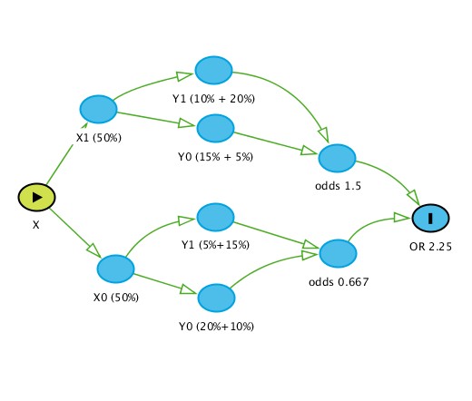
This figure demonstrates the flow of stratification (X is the exposure and Y is the outcome) and clearly the unconditional OR (2.25) differs from the ones conditioned on Z (2.67) and the reason is quite clear - the unconditional OR is subject to how Z redistributes across strata of X given that both X and Z are prognostic for Y. Thus the OR of 2.25 is simply an “average” OR when we do not measure other prognostic factors and Z while the conditional OR is the “average” OR when we do not measure other prognostic factors except Z. Thus we can agree that non-collapsibility implies that this is a true effect measure and collapsibility implies otherwise.

Having introduced this lets analyze the Greenland example using logistic regression and a sample size of one million:

We get the ORs as expected
1.X 2.67
1.Z 6
X#Z 1
_cons 0.25 (baseline odds)

These are the same results from Greenland
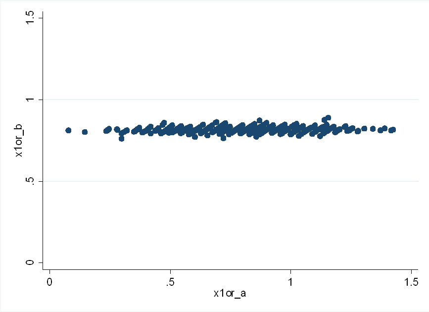
Now lets randomly select a sample of 400 from this million participants and run the regression again

We get the ORs as follows
1.X 1.30
1.Z 2.74
X#Z 2.76 (P=0.022)
_cons 0.46 (baseline odds)

Without the interaction we get back to a closer estimation of reality which is:

1.X 2.13
1.Z 4.35
_cons 0.35 (baseline odds)

Each time we select a sample of 400 this interaction term varies widely. The average OR remains reasonable without the interaction but seems ridiculous with it and the interaction is basically a consequence of random redistribution of strata so does this mean that interactions are not meaningful since they are simply due to random error?

[Sander]

I can’t make sense of your comment that the
“The average OR remains reasonable without the interaction but seems ridiculous with it”:
The simple geometric mean OR with the product term is the square root of 1.30*(1.30*2.76) which is 2.16, nearly equal to the no-product OR of 2.13 and hardly unreasonable given the random error and that the target (the conditional OR) is 2.67.

[s_doi]

I meant this more in the sense of a “typical” OR for X (say)
So to be more specific say we get a sample like this and we do not have the hindsight of the whole population.
In these situations we will get a more realistic OR (for X) by ignoring the interaction term even if there is a poorer model fit. This also links to the other question posted - could that interaction also be due to random error too? When and how do we know when an interaction is meaningful or should be ignored?

Edit: I get the point that the OR lies between 1.3 and 1.3*2.76 and that is what surfaces without the interaction term but then the question is what is typical for X here and how do we know - it certainly does not vary in effect by strata of Z so why bother with the interaction and how do we justify this?

[Sander]

I’m still unclear about what you are asking.

As you said, in your example the underlying Z-specific OR is constant because you set it up that way. More generally, if you knew that it was constant and your goal was only to estimate ORs, there would be no reason to use the product term. But in real problems there is no reason to expect the OR to be constant - what biologic process would lead to that and how could we be certain it held?

At most we can say we might expect the OR to be less varying across Z than (say) a variation-constrained measure like the RD. To say there is no “interaction” (product term) just because p>0.05 is confusing absence of information about how the X-Y OR varies with information that the X-Y OR does not vary. That is just the 2nd-order version of the nullistic fallacy (confusing absence of evidence with evidence of absence, i.e., standard JAMA editorial policy).

If you are asking how in real problems we should use product terms, you’d have to first have to state the goal of your analysis and provide some sense of error costs. If that goal were to come up with ‘accurate’ Z-specific estimates, you’d have to state of what and why. OR? RR? RD? The answer could vary by choice; I’d want to compute the RR and RD from the fitted risks from a very flexible model. At realistic study sizes this can become a delicate problem in patient-specific clinical risk prediction; hierarchical (e.g., empirical-Bayes or partial-Bayes) estimation might be called for. There are some good modeling books out there for risk prediction including Frank’s.

Modeling can be easier if you only want an average of the Z-specific measures over Z, or only want a marginal average. For averaging, just using the fitted probabilities from most any good-fitting model in place of the data proportions might well suffice. Some old citations for that include Ch. 4 and 12 of Bishop YMM, Fienberg SE, Holland PW. Discrete multivariate analysis: theory and practice. Cambridge, MA: MIT Press, 1975, and Greenland S, Maldonado G. The interpretation of multiplicative model parameters as standardized parameters. Statistics in Medicine 1994;13:989-999.
More modern model-averaging methods are based on Robins’ g-computation formula, e.g., IPTW and doubly robust estimators as in the new Causal Inference book by Hernan & Robins.

See Ch. 21, p. 435 onward of Modern Epidemiology 3rd ed. 2008 for a very quick introduction to hierarchical and model-based risk prediction and averaging, along with detailed citations.

[s_doi]

Thanks, if I understand you correctly, and we assume X is the treatment (say A vs B) and Y is the outcome say recovery, then you are saying that the subgroup effect by Z needs to be modeled properly for any substantive interpretation to be valid otherwise it should be ignored.

What is proper seems unclear to me. This paper that discusses predictive regression approaches to HTE analysis says that “modeling such interactions can result in serious overfitting of treatment benefit” but did not seem to think there was any real solution (for effect modeling). Rothwell suggests that the only sure way is replication. Then why bother with subgroup analyses and effect modeling in such studies that we see all the time in reports of clinical studies and will the correct answer to the question raised by colleagues in the linked post be that its spurious until replicated?

[Sander]

The new BMC MRM review you linked looks like a good technical resource, with many valuable cites including materials by Harrell and by Steyerberg. A limitation of the paper however is that it does not deal with the complex issue of error costs.

I still find some of your comments puzzling, e.g., I did not see where it said they “did not think there was any real solution.” I thought it said that they had not found a lot of field testing among proposed solutions, hence they could not make clear recommendations. It also touched on the difficulty of constructing valid field-evaluation criteria (as opposed to artificial math-analytic or simulation criteria).

As I mentioned at the start, the notion that these issues should lead one to treat a product term as “spurious until replicated” is just fallacious 2nd-order nullism. But ignoring product terms gains some support from statistical theory via this valid point: Suppose in a hierarchical/empirical-Bayes context we are willing to take the main-effects only model as our prior-mean model or shrinkage manifold for penalization. Then at sample sizes typical of RCTs we’ll often (if not usually) find that the covariate-specific predictions get shrunk almost if not completely to those from that model (depending on the type of shrinkage used).

Practically speaking this means that, unless we have a lot more (data or prior) information for each covariate combination than typical, our best bet will be to just apply the main-effects-only model to predict effects. Unfortunately, that advice stems from the loss function implicit in the method used (e.g., MSE loss for coefficients when using Gaussian shrinkage; MAE loss when using lasso). These coefficient loss functions make no sense when translated into clinical reality, and so I do not believe that standard statistical advice is the best we can do in any given case. Nor do good clinicians: At the very least they read the product insert to avoid using a medicine on those at risk of identified potential serious side effects, and attempt to calibrate dosing according to guidelines and patient characteristics (typically age, weight, sex), and then monitor patient reaction.

So the reality is that good clinicians use effect-modification information all the time! They just do so based on guidelines reported from previous trials, as summarized in the product information, plus some common sense that the effective dose for a 100 lb adult is likely less than for a 250 lb adult. The technical complexities come from attempts to refine guidelines using statistical algorithms that ignore such background information, when there simply isn’t enough data information to compensate for that ignorance.

In sum, on this topic I think the gap between theory and practice remains enormous due to lack of real data to evaluate procedures, and lack of validated information to guide practice in the face of that reality. Automated one-size-fits-all recommendations on how to proceed are at best administrative heuristics to get on with practice, and at worst are sheer statistical quackery (e.g., declaring modification absent because p>0.05 for a product term, when at most that means the direction of modification is ambiguous).

[s_doi]

That’s my impression of where the authors were heading . Its much clearer in my mind now and you are right - there needs to be a more nuanced view taken regarding these product terms and of course some basic understanding of the underlying context.

[f2harrell]

One narrow comment to add to this excellent discussion: Because of the limited information content in the data that would allow for full estimation and inference about differential treatment effects (interactions on a scale for which such interactions might be absent), there is a place for pre-specification of prior knowledge or constraints about interaction effects. Injecting skepticism in prior distributions for interaction effects is a logical place to do this, as discussed in detail here.

[s_doi]

Perhaps I can take this further by asking another question. For now lets stick with this example of a binary outcome and categorical prognostic variables. Say z indicates gender.

1. Would it be considered okay to say that there is modification of the effect of x on y by gender if the rate of change in probability of y per unit change in x differs by gender?
2. If so, then does that not make the link of interest in a glm (log or identity) redundant and therefore the question of there always being an interaction (on some scale) when both x and z are prognostic for y is no longer meaningful?

[f2harrell]

When effect modification is exactly zero, the scale on which it is quantified does not matter. In all other cases, the scale matters. We like scales for which it is possible that effect modification is zero even when a variable such as z has an effect everywhere, hence the popularity of scales without range restrictions, such as logit and probit.

Rate of change of probabilities doesn’t tell us anything special, and is not accepted as a measure. Contrast that with the one rate that we do find useful, which relates to the limit of a conditional probability as the time increment goes to zero: the hazard rate.

So I’ll stick to the linear predictor scale in GLMs and beyond.

[s_doi]

Thanks, so if I understand correctly, you are saying that the link transform (log or logit) to a continuous scale (of the probabilities of the levels of y) that is unbounded is what is important for defining an interaction while the probabilities themselves (of the levels of the categorical response variable y) is not accepted. This would mean that an interaction (as we currently define it) is a function of the transformed scale (where the parameters are linearly specified) versus the natural scale where the model is meaningfully interpreted into clinical practice.

In the glm the marginal effects quantify the interaction on the natural scale and characterize the rate-of-change of y for a change in x holding all else constant. The glm coefficients do not capture the marginal effects in the natural scale but rather linear change on the transformed log/logit scale. Why are epidemiologists not defining an interaction as change in the marginal effect for a focal variable for a change in the moderating variable? Would this not completely resolve the whole question of interactions being different on one scale or another and indeed unify this area because it makes it binary - an interaction will either be present on all scales or absent on all scales and the scale itself just becomes a tool.

[f2harrell]

I do not find it valuable to emphasize change on a marginal scale. But think of it more generally: For clinical interpretation when the outcome is binary so that time is not involved, the patient needs to see two quantities: the absolute risk if untreated and the absolute risk if treated. The difference between these two (which does not actually need to be computed) will vary greatly with baseline risk whether or not an interaction is in the model. So you can de-emphasize the interaction discussion and say that effects on the linear predictor (link) scale are convenient means to an end. They give us parsimony, and they give rise to accurate predictions on any scale of interest. Proper inclusion of interactions on the, say, logit scale, when needed, is necessary to give accurate estimates on any scale.

[f2harrell]

To me this is worse than counterintuitive. It is something that causal inference experts, with all the amazing good things they are doing, have perpetrated on us. They tend to have a deep hatred of odds ratios for reasons that still escape me. I embrace odds ratios, use them as a basis for modeling, then convert the model to any scale that anyone needs. Effect modification must be measured on a scale for which it is mathematically possible that effect modification can be zero. Otherwise effect modification as a purely mathematical construct on the absolute risk scale will be misrecognized as a biological structural effect.

[s_doi]

I agree fully - the critique of the odds ratio for being non-collapsible is a point in case. Its this particular property of the OR that makes it mathematically possible that effect modification can be truly zero when it is zero and I agree that effect modification seems to be a purely mathematical construct on other scales. That’s why I attempted to raise the idea of returning to the natural scale for interaction effects previously - to avoid misinterpreting collapsible measures although I really doubt if the RR is a measure of effect that needs salvaging .

[s_doi]

Thanks - good to get your perspective on this. I am trying to clarify a few concepts in my mind surrounding interactions and their relationship to causal effects. Hernan says in his book (section 4.1) that “We do not consider effect modification on the odds ratio scale because the odds ratio is rarely, if ever, the parameter of interest for causal inference.” This is certainly counter-intuitive given the non-portability of RRs and the irrelevant statistical interactions on the log scale (in glm’s) consequent on the latter problem. I will have to think a bit more about this but clearly the views are divergent on this topic.

I deleted this post above and am re-posting here to change the term “transportable” to “portable” as they seem to connote different ideas to different researchers.

I thought this is a good place to continue a discussion from a previous thread about product terms. So in the plot below, Z is a random binary variable with no prognostic implication for Y created by deleting Z from the dataset above and recomputing it such that there are 200 observations assigned to each category (0, 1) completely at random. The results of OR(XY) with (a) and without (b) the product term is indicated in the plot below:

Despite only random error being at play, the product term has a wide variability around zero (its true value on the logit scale) and thus had we considered systematic error this would have been even worse.

Rekkas et al state that *"Treatment effect modeling methods focus on predicting the absolute benefit of treatment through the inclusion of treatment-covariate interactions alongside the main effects of risk factors. However, modeling such interactions can result in serious overfitting of treatment benefit, especially in the absence of well-established treatment effect modifiers.

I think this is well demonstrated in the plot above.

they then say that “Penalization methods such as LASSO regression, ridge regression or a combination (elastic net penalization) can be used as a remedy when predicting treatment benefits in other populations”.

I will try out LASSO logit regression and see what happens to the simulation above and report back

[s_doi]

Here goes another attempt (may be wrong so if so please say so and point me in the right direction). We take the same simple example of three binary variables: outcome (Y), intervention (X) and third variable (Z) with X and Z both prognostic for Y.

First I start with the relationship of the exponentiated product term (PT) to the area under the curve (AUC) in logistic regression where delta stands for “incremental”

We can then run a bootstrap to get the CI for delta area and if the lower CI is less than an arbitrary value (say 0.6) then we drop the PT as random error even if the P for interaction is much less than 0.05

In Stata the bootstrap would be run as follows:

bootstrap (sqrt(exp(_b[1.x#1.z]))/(1+sqrt(exp(_b[1.x#1.z])))): logit y i.x##i.z

Any thoughts?

NB: Applies to observed PT>1 for observed PT<1 use 1/PT

[Pavel_Roshanov]

This is a very interesting discussion.

It seems to me that the problem of non collapsibility is a big problem for subgroup analyses with unadjusted OR and HR as the estimator of effect because subgroups have different distributions of important covariates. When specific to a subgroup, the hazard ratio is conditional on the covariate distribution of that subgroup and therefore will be different than the overall hazard ratio and from the hazard ratio of the comparator subgroup.

Does this not create a significant problem for subgroup analyses?

and even when “adjusted”, it seems to me that within-subgroup homogeneity of treatment effect is still assumed

[s_doi]

I think the important point was made by Frank above when he said “Effect modification must be measured on a scale for which it is mathematically possible that effect modification can be zero. Otherwise effect modification as a purely mathematical construct on the absolute risk scale will be misrecognized as a biological structural effect.”

In a subgroup analysis (say M and F) and assuming the subgroup variable is prognostic for the outcome then you have three effects:
a) In M
b) In F
c) Marginal
All three are different groups of people and must have different effects and saying that covariate adjustment or stratification leads to decreased precision for the treatment effect estimator is not really true because these are estimators of different estimands.

What follows is that noncollapsibility is the desired behavior of a good effect measure because the effect reflects the covariate distribution of the particular group of interest and thus the marginal estimate must be tilted towards the null compared to a conditional estimate if the conditioning is on a covariate prognostic for the outcome (regardless of confounding or not). So in summary, only a noncollapsible effect measure can be useful for subgroup analyses as they only accurately reflect changes in the covariate structure of the data in terms of impact on the main effect of treatment.

Keep in mind however that artifacts of the data can easily pop up as a product term in a GLM with a p for interaction <0.01 for example and thus even with noncollapsible measures starting from the position of homogeneity is perhaps better

[Pavel_Roshanov]

Using a relative instead of absolute measure makes sense, but I am still uncertain whether this measure should be an RR or a noncollapsible OR/HR. I recognize that high baseline risks put constraints on the RR, but most baseline risks in medicine are low and most effects are small.

“effect measure can be useful for subgroup analyses as they only accurately reflect changes in the covariate structure of the data”

This is an interesting approach, but then you say “even with noncollapsible measures starting from the position of homogeneity is perhaps better” presumably because changes in the covariate structure are problematic and muddy the interpretation of effect modification by the variable of interest.

[s_doi]

I am not sure that covariate structure is the issue with modifiers as you have put it
Best to give a numerical data example in a table and we can discuss how the interpretation varies based on choice of RR or OR.