Interpreting the results of two non-inferiority trials

This is my first post on datamethods so I hope it is appropriate and of some interest.

Colleagues of mine recently published a trial as one of two back-to-back papers in the Lancet (1, 2). The trials were addressing the same clinical question and reported almost identical hazard ratios for the primary outcome. Despite the similar results the conclusions in terms of the implications for clinical practice were the opposite. They asked me to comment on the results.

As I am no expert on the analysis of nuanced interpretation of RCTs, even less so for those with a non-inferiority question, I thought I’d put my thoughts in a public forum and get others opinions. My interpretations may be way off kilter!

Both trials were non-inferiority trials evaluating whether 6-months of trastuzumab therapy was equivalent to the standard 12-months treatment in HER2-positive early breast cancer. Shorter treatment could provide similar efficacy while reducing toxicities and cost. The primary end point was disease free survival in both trials. Four thousand and eighty-nine patients were randomised in the PERSEPHONE trial and followed for a median of 5.4 years (512 events) and 3,384 were randomised in the PHARE trial and followed for a median of 7.5 years (704 events). The hazard ratio for 6-months compared to 12-months was 1.07 (0.93 – 1.24) in PERSEPHONE and 1.08 (0.93 – 1.25) in PHARE (inappropriately described as disease-free survival in the 12-month group versus the 6-month group).

The conclusions were: “ We [PERSEPHONE trialists] have shown that 6-month trastuzumab treatment is non-inferior to 12-month treatment in patients with HER2-positive early breast cancer, with less cardiotoxicity and fewer severe adverse events. These results support consideration of reduced duration trastuzumab for women at similar risk of recurrence as to those included in the trial .” And, “ The PHARE study did not show the non-inferiority of 6 months versus 12 months of adjuvant trastuzumab. Hence, adjuvant trastuzumab standard duration should remain 12 months.

Given these apparently diametrically opposite conclusions to what are similar results, how should the totality of the data be interpreted.

In PERSEPHONE, non-inferiority was predefined as a less than 3% absolute difference in disease-free survival at 4 years. The observed 4-year survival was 0.894 in the 6-month group compared to 0.898 in the 12-month group. Based on the observed cumulative risk in the 12-month group of 0.102 a 3% absolute difference would be 0.132 which would correspond to a hazard ratio of 1.32. Non-inferiority in PHARE was defined as a hazard ratio of less than 1.15. Based on the 5-year survival of 0.892 in the 12-month group this would be equivalent to a 1.5% absolute difference at 5 years or a difference of 1.3% at 4 years.

It is immediately apparent that a difference in the definition of non-inferiority gives rise to the potential for different conclusions from similar data. There is little in the published reports to justify either non-inferiority margin although non-inferiority based on a relative value (as used in PHARE) seems inappropriate for clinical decision making given that it is a truism that clinical decisions ought to be based on absolute changes in risk, not relative changes.

Greater certainty might be obtained from combining the results of the two studies, which would provide more precise estimates of the difference in effect in the 6-month and 12-month groups. Using a fixed effects model, the meta-analysis hazard ratio is 1.075 (0.970 – 1.19) and the average cumulative survival at 4 years in the 12-month group is 0.905. These parameters can be used to plot the probability density for the absolute risk difference in survival at 4 years (Figure 1).

Figure 1: The probability density for the predicted absolute difference in disease-free survival at 4 years based on meta-analysis of the results from both trials
image

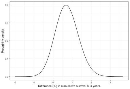
The point estimate is an absolute difference in disease free survival of 0.7%. The PHARE trialists did not specify non-inferiority on an absolute scale but there is a 16 per cent chance that the difference is greater than 1.3 per cent (the approximate absolute difference equivalent to a relative hazard of 1.15). The probability that the difference is 3 per cent is just 0.02%. There is an 80 per cent chance that the difference is less than 1.2 per cent and a 12 per cent chance that outcome is more favourable in the 6-month group.

If one evaluated these trials as an investigation of the superiority of 12-months treatment compared to a hypothetical standard of 6-months treatment the one-sided P-value for superiority would be 0.12 and the standard conclusion would be that 12-months is not superior to 6-months.

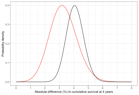
An alternative approach to evaluation would be to consider the likely effect of 6-months and 12-months trastuzumab and compared to no targeted therapy. Four studies have reported on the benefit of 12-months trastuzumab on disease free survival (3-6). A fixed effects meta-analysis of the reported hazard ratios for these studies gives a hazard ratio of 0.68 (95% CI 0.63 – 0.74). The probability distribution for the predicted absolute benefit of 12-months traztusumab at four years is shown in Figure 2 (black line). If we now estimate the predicted absolute benefit of 6-months therapy from the product of the hazard ratio for 12-months therapy and the 6-month versus 12-month comparison the probability distribution for the absolute benefit at four years is the red line in Figure 2. This shows that there remains substantial uncertainty in the likely effect of 6-months trastuzumab therapy.

Figure 2: Comparison of the probability distribution for the absolute benefit of 12-months trastuzumab (black) or 6-months trastuzumab (red) compared to no trastuzumab

image

In conclusion, whether or not 6-months adjuvant trastuzumab should be considered inferior to 12-months depends on the definition of inferiority and on how certain one wishes to be regarding any specified threshold.

References

  1. Earl HM, Hiller L, Vallier AL, et al. 6 versus 12 months of adjuvant trastuzumab for HER2-positive early breast cancer (PERSEPHONE): 4-year disease-free survival results of a randomised phase 3 non-inferiority trial. Lancet 2019; 10.1016/S0140-6736(19)30650-6.

  2. Pivot X, Romieu G, Debled M, et al. 6 months versus 12 months of adjuvant trastuzumab in early breast cancer (PHARE): final analysis of a multicentre, open-label, phase 3 randomised trial. Lancet 2019; 10.1016/S0140-6736(19)30653-1.

  3. Spielmann M, Roche H, Delozier T, et al. Trastuzumab for patients with axillary-node-positive breast cancer: results of the FNCLCC-PACS 04 trial. J Clin Oncol 2009;27(36):6129-34.

  4. Slamon D, Eiermann W, Robert N, et al. Adjuvant trastuzumab in HER2-positive breast cancer. N Engl J Med 2011;365(14):1273-83.

  5. Perez EA, Romond EH, Suman VJ, et al. Trastuzumab plus adjuvant chemotherapy for human epidermal growth factor receptor 2-positive breast cancer: planned joint analysis of overall survival from NSABP B-31 and NCCTG N9831. J Clin Oncol 2014;32(33):3744-52.

  6. Joensuu H, Bono P, Kataja V, et al. Fluorouracil, epirubicin, and cyclophosphamide with either docetaxel or vinorelbine, with or without trastuzumab, as adjuvant treatments of breast cancer: final results of the FinHer Trial. Journal of Clinical Oncology 2009;27(34):5685-92.

7 Likes

What a wonderful post Paul. I sincerely hope that those out there who are experienced with non-inferiority trials will respond. My general take is that study designers are given too much latitude in selecting non-inferiority margins, and that there is something to be said for not using statistical tests against what is often in effect a “straw man” but instead to use Bayesian methods to compute the posterior probability that the true hazard ratio exceeds or is less than r for all possible values of r. Short of that, relying on the published confidence interval rather than a statistical test would be an improvement IMHO.

5 Likes

That researchers have to torture the classical hypothesis testing framework in order to provide evidence in favor of the null, is enough to convince me that likelihood methods (if a full Bayesian treatment can’t be done) would be better.

This paper by SJ Wang and Jeffrey Blume describe a rational approach to the problem.

2 Likes

The first thing I would look for is how rigorously the trials were conducted, in particular, how much did the patients adhere to the 12-month treatment? If the trial is sloppy, the ITT analysis will penalize the new treatment in a superiority trial but favor the new treatment in a non-inferiority trial. This is one of the reasons why >80% of non-inferiority trials demonstrated non-inferiority as discussed here.

Also, I have to say that a hazard ratio of 1.32 is quite a lenient margin. I prefer using ratios (such as HR) in these calculations as they tend to be more portable than absolute differences.

5 Likes

Thanks.

I think these were both well-conducted trials. The therapy is given parenterally so deviations from ITT will be very limited. E.g. in PERSEPHONE 86% planned doses were given (90 v 84 for 6- and 12-month arms). Reasons for not giving were mainly cardio-toxicity.

I agree that the NI margin in PERSEPHONE is quite lenient. I accept that the relative parameter is more portable, but for clinical decision making absolute risks are more relevant. On the other hand the absolute risk when applied outside the context of a clinical trial may be inappropriate and under those circumstances, appying the RH to a different cumulative risk might be more appropriate.

2 Likes

A further thought. While the trial design pre-specifies a non-inferiority margin I wonder how often the trialists genuinely discuss and agree this before they have any idea of the sample size requirement. Or do people work out what sample size is going to be possible and then effectively work out the NI margin from that.

If small (differences in) effects are clinically important non-inferiority trials are all but impossible as the sample size to get a very precise estimate becomes prohibitive.

2 Likes

Yes, I’ve seen researchers calculate the NI margins based on how many patients can be pragmatically accrued. This is a version of what @AndrewPGrieve calls “resource sizing” and it has many issues described here.

2 Likes

A major problem seems to be that leaders of particular clinical trials are selecting non-inferiority margins, and it should be patients and practicing physicians who should be choosing them.

5 Likes

Really great post highlighting the problems of non-inferiority studies, especially when using NHST. Reporting probability densities seems a much better way to show the available information.

As a clinician with a love for epidemiology and (Bayesian) statistics I am interesting in the statistical (R?) code used for the post, any chance this can be made available for personal learning purposes?

I’ll send the R-code once I’ve time to tidy up and sure it’s sensibly annotated.

1 Like

Thanks! Much appreciated!

Here is my code. Let me know if questions or if you spot an error.

library(tidyverse)
library(meta)

Enter data from trastuzumab trials for 12-months + chemo v chemo

traz <- tribble(~study, ~year, ~number, ~median_fu, ~hr, ~lcl, ~ucl, ~endpoint,
“Slamon”, 2011, 3222, 5, 0.64, 0.50, 0.82, 1,
“Slamon”, 2011, 3222, 5, 0.63, 0.49, 0.82, 2,
“HERA”, 2017, 3399, 11, 0.76, 0.68, 0.86, 1,
“HERA”, 2017, 3399, 11, 0.74, 0.64, 0.86, 2,
“B31/N9831”, 2014, 4064, 8.4, 0.60, 0.53, 0.68, 1,
“B31/N9831”, 2014, 4064, 8.4, 0.63, 0.54, 0.73, 2,
“PACS04”, 2009, 528, 3.9, 0.86, 0.61, 1.22, 1) >
mutate(log_hr = log(hr),
se = (log(ucl)-log(lcl))/(2*qnorm(.975))
)

Do fixed effects meta-analysis for disease free survival (endpoint=1)

traz.meta <- metagen(log_hr, se,
backtransf=TRUE,
studlab=study,
data=filter(traz, endpoint==1))

forest(traz.meta, studlab=TRUE,
sortvar = traz.meta[[‘w.fixed’]],
col.fixed=‘red’,
study.results=TRUE,
rightcols=c(“effect”, “w.fixed”),
leftcols=c(“studlab”),
backtransf=TRUE)

Enter data for 6months v 12-months trastuzumab

df <- tribble(~study, ~subtype, ~hr, ~lcl, ~ucl,
“Earl”, “All”, 1.07, 0.90, 1.27,
“Earl”, “ER+”, 0.96, 0.76, 1.20,
“Earl”, “ER-”, 1.26, 0.97, 1.64,
“Earl”, “Concurrent”, 1.53, 1.16, 2.01,
“Earl”, “Sequential”, 0.84, 0.68, 1.06,
“Pivot”,“All”, 1.08, 0.93, 1.25,
“Pivot”, “ER+”, 1.07, 0.87, 1.31,
“Pivot”, “ER-”, 1.08, 0.88, 1.35,
“Pivot”, “Concurrent”, 1.05, 0.86, 1.28,
“Pivot”, “Sequential”, 1.11, 0.89, 1.39) >
mutate(log.hr = log(hr),
se = (log(ucl)-log(lcl))/(2*qnorm(.975)))

Meta-analysis for results by subtype

m <- metagen(log.hr, se, data=df, byvar=subtype, comb.random=FALSE)

meta.out <- cbind(m[[“bylevs”]], m[[“TE.fixed.w”]], m[[“seTE.fixed.w”]])

Save outputs as a tibble

meta.out <- as_tibble(meta.out) >
rename(subtype=V1, log.hr=V2, se=V3) >
mutate(log.hr=as.numeric(log.hr),
se=as.numeric(se)) >
mutate(study=“Combined”,
hr=exp(log.hr),
lcl = exp(log.hr - qnorm(.975)*se),
ucl = exp(log.hr + qnorm(.975)*se))

Combine study specific results with meta-analysis results

df <-rbind(df, meta.out)

Inpute cumulative survival estiamtes at 6 and 12 months for the two studies

cs12.perse.4 <- 0.898
cs6.perse.4 <- 0.894
cs12.phare.5 <- 0.892
cs6.phare.5 <- 0.884

Estiamte cumulative incidence and average annual incidence for PERSEPHONE

ci12.perse.4 <- -log(cs12.perse.4)
i12.perse <- ci12.perse.4/4
ci6.perse.4 <- -log(cs6.perse.4)
i6.perse <- ci6.perse.4/4
hr.perse <- i6.perse/i12.perse

Estiamte cumulative incidence and average annual incidence for PHARE

ci12.phare.5 <- -log(cs12.phare.5)
i12.phare <- ci12.phare.5/5
ci6.phare.5 <- -log(cs6.phare.5)
i6.phare <- ci6.phare.5/5
hr.phare <- i6.phare/i12.phare

Estimate of the 4 year survival in combined data

Strictly speaking this ought to be a weighted average

i12.comb <- (i12.perse + i12.phare)/2
cs12.comb <- exp(-4*i12.comb)

Estimate the non-inferiority absolute diff in combined data

for absolute difference at 4 years

ni.diff.phare <- cs12.comb - exp(-4i12.comb1.15)

Estimate of the pooled hazard ratio from first principles

Fixed effects pooled odds ratio

hr1 <- 1.07
lcl1 <- 0.93
ucl1 <- 1.24
log.hr1 <- log(hr1)
se1 <- (log(ucl1)-log(lcl1))/(2*qnorm(.95))

hr2 <- 1.08
lcl2 <- 0.93
ucl2 <- 1.25
log.hr2 <- log(hr2)
se2 <- (log(ucl2)-log(lcl2))/(2*qnorm(.975))

log.hr.hat <- (log.hr1/(se1^2) + log.hr2/(se2^2))/(1/se1^2 + 1/se2^2)
se <- 1/((1/se1^2 + 1/se2^2)^.5)
z <- log.hr.hat/se
p <- pnorm(-z)
hr.hat <- exp(log.hr.hat)
hr.lcl <- exp(log.hr.hat - qnorm(.975)*se)
hr.ucl <- exp(log.hr.hat + qnorm(.975)*se)

Function for probability that a given difference is greater

than a specific difference given cumulative survival in one

group, hazard ratio and LCL hazard ratio

p.func <- function(diff, cs.group1, hr.obs, lcl.obs) {
se.log.hr <- (log(hr.obs) - log(lcl.obs))/qnorm(.95)
cs.group2 <- cs.group1 - diff/100
ci.group1 <- -log(cs.group1)
ci.group2 <- -log(cs.group2)
hr <- ci.group2/ci.group1
z <- (log(hr)-log(hr.obs))/se.log.hr
pnorm(-z)
}

Probability of difference at 4 years being greater than 3%

p.func(diff=3, cs.group1=cs12.comb, hr.obs=hr.hat, lcl.obs=hr.lcl )

Probability of difference at 4 years being greater than %

p.func(diff=1.3, cs.group1=cs12.comb, hr.obs=hr.hat, lcl.obs=hr.lcl )

p.func(diff=2, cs.group1=cs12.comb, hr.obs=hr.hat, lcl.obs=hr.lcl )

1-p.func(diff=0, cs.group1=cs12.comb, hr.obs=hr.hat, lcl.obs=hr.lcl )

d.func <- function(diff, cs.group1, hr.obs, lcl.obs) {
se.log.hr <- (log(hr.obs) - log(lcl.obs))/qnorm(.95)
cs.group2 <- cs.group1 - diff/100
ci.group1 <- -log(cs.group1)
ci.group2 <- -log(cs.group2)
hr <- ci.group2/ci.group1
z <- (log(hr)-log(hr.obs))/se.log.hr
dnorm(z)
}

q.func <- function(prob, cs.group1, hr.obs, lcl.obs) {
se.log.hr <- (log(hr.obs) - log(lcl.obs))/qnorm(.95)
z <- -qnorm(prob)
hr <- exp(z*se.log.hr + log(hr.obs))
cs.group2 <- exp(log(cs.group1)*hr)
diff <- (cs.group1 - cs.group2)*100
diff
}

Plot the estimated absolute difference in cum survival

ggplot(data.frame(diff = c(-2, 3.67)), aes(x=diff)) +
stat_function(fun=d.func,
args=list(cs.group1=cs12.comb,
hr.obs=hr.hat,
lcl.obs=hr.lcl)) +
geom_vline(xintercept=1.3, linetype=“dashed”) +
scale_x_continuous(breaks=seq(-2,3,1),labels=seq(-2,3,1)) +
theme_bw() +
labs(x = “Absolute difference (%) in cumulative survival at 4 years”,
y = “Probability density”)

Plot the estimated difference between 6-month or 12-months v no trastuzumab

ggplot(data.frame(diff = c(-0, 20)), aes(x=diff)) +
stat_function(fun=d.func,
args=list(cs.group1=0.63, #cs12.comb,
hr.obs=exp(.307),
lcl.obs=exp(.307-0.0661*1.96)),
color=‘red’) +
stat_function(fun=d.func,
args=list(cs.group1=0.63, #cs12.comb,
hr.obs=1.46,
lcl.obs=1.35),
color=‘black’) +
scale_x_continuous(breaks=seq(0,20,1),labels=seq(0,20,1)) +
theme_bw() +
labs(x = “Absolute difference (%) in cumulative survival at 10 years”,
y = “Probability density”)

6 Likes

Thank you very much, I will look into the code and try to learn from it, great work!

I’ve got one question: you calculated the probability density for predicted absolute difference in Figure 1. I have difficulty interpreteting these numbers and the interpretation, for instance such as in the sentence “there is a 16 per cent chance that the difference greater than 1.3 per cent”. Are these true probabilities, comparable to those resulting from a Bayesian analysis? If so, is there any underlying prior used? If not, how should I interpret these percentages?
The figure (both 1 & 2) seems a wonderful way to present the results of the trial, so I am wondering why it is not used more often in RCT papers, is there any reason for this?

This is not a probability distribution based on a formal Bayesian analysis because it does not have any prior attached. It is simply based on the point estimate and 95% CI of the estiamted hazard ratio and then is converted into an absolute risk rather than relative risk. If one assumes a prior for log hazard ratio as a normal distribution ~ (0.049, 0.018) (equivalent to a HR of 1.15 with the upper 97.5% limit of 1.3) then the observed and posterior distribution almost overlap. I’d need to do a bit more to get a more sensible prior distribution.

I am not the person to ask about the presentation of results for non-nferiority trials. This is the first time that I have ever thought about the issue.

1 Like