Add to the plot the confidence and for the difference in the two curves, which would better support your implication that there is signal there that a PH model missed.
3 Likes
I was curious and made the analysis you suggest, for the Keynote-061 trial… the authors considered it negative, literally concluding that pembrolizumab does not increase overall survival.
https://www.thelancet.com/journals/lancet/article/PIIS0140-6736(18)31257-1/fulltext
Instead, on this plot, I show the difference of survival with the survdiffplot function of the rms package.
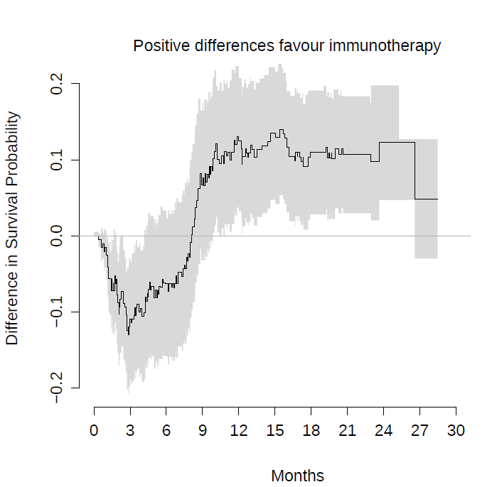
This is the same conclusion as in figure 4 of our article with a spline-based model.
Sadly, because these studies have been declared negative, patients do not benefit from these strategies. Worse, clinicians don’t discuss the problem of crossing hazards. However, among my colleagues I have received quite a lot of criticism. The opinion of the clinicians is that to reanalyse clinical trials, even if they are poorly designed, is always to go fishing for p-values. So it has occurred to me to reproduce these analyses with a Bayesian Royston-Parmar model, which does not require pre-specifying the time point at which the survival difference is measured. The question would be how to pre-specify the prior for the number of parameters of the splines… Another Bayesian option would be the equivalent of survdiffplot My idea is to propose to completely abandon frequentist hypothesis tests, which lead to a dead end.
Instead, a Bayesian estimate of survival differences could be shown with their credibility intervals at all points at once. Instead of a decision criterion, the clinician could qualitatively judge the entire curve. I think this goes in the direction of the spirit of times. The FDA is actually accepting promising drugs only with phase I/II trials in orphan indications. So the Bayesian analysis would explicitly address this real concern of the regulators.
2 Likes
The graphic above conveys something nice for me. By not capturing the crossing curve as expected, the differences in survival predicted by Cox’s model for late time points are biased, being smaller than the real ones. This beautifully illustrates, in my oncological opinion, the loss of statistical power that you risk if you use Cox’s model for this data. If you add the super convoluted hierarchical designs, it is almost impossible that any of these trials could be positive.
1 Like
Really nice displays that give ammunition that the PH assumption really mattered here.
You raise some huge points that should be discussed for a while. Regarding trustworthiness of reanalysis, I’m feeling more and more that if we use self-penalizing approaches we should be granted leeway. A rational approach that is self-penalizing is having 2 parameters for treat: treatment main effect + tx by log(time) interaction. Then estimate treatment effect as a function of time with highest posterior density intervals.
This begs the question of which treatment is better. That depends on the patient’s utility function. There is no single answer. But presenting results for all times (whether log hazard ratio vs. time or differences in cumulative incidences) is a great way to communicate this.
5 Likes
For many oncologists one of the most bizarre passages in the history of medicine occurred in this article:
Mok et al wrote:
The median progression-free survival was 5.7 months in the gefitinib group and 5.8 months in the carboplatin–paclitaxel group […]. The study met its primary objective of demonstrating noninferiority and showed the superiority of gefitinib as compared with carboplatin–paclitaxel for progression-free survival […]. Apparently they published in NEJM that 5.7 is more than 5.8 months.
Here, beyond the analysis, the important thing is that the crossing hazards always translate the presence of a strong effect-modifying factor. In the case of Mok et al, EGFR mutations. For immunotherapy there is certainly a strong predictive factor yet to be discovered, which is fascinating.
If I understood correctly, you suggest using the formula treatment + treatment * time in a survival model. That could work for non-PH scenarios.
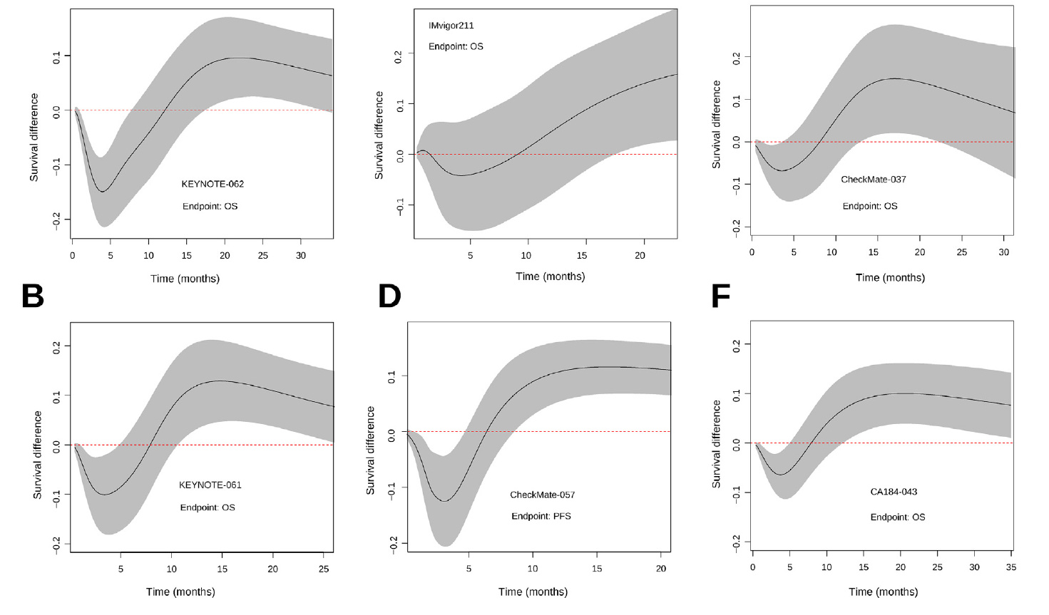
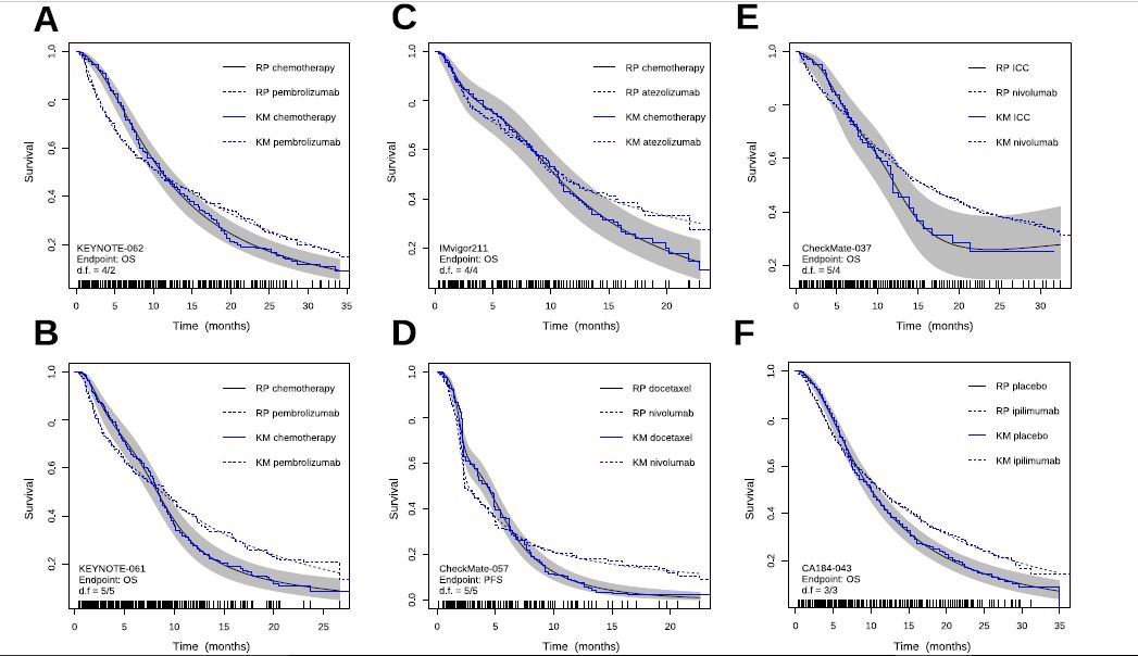
My doubt is how to code the crossing hazards with only two degrees of freedom. My experience with the Royston-Parmar model was that 5+5 degrees of freedom were required to capture the behavior of the more complex examples. Below I show the plots we made by comparing the model estimates with the KM curves. With less degrees of freedom the Royston-Parmar model, which is quite flexible, worked quite worse. If you look at it, the curves do some really weird things.
4/2 is looking pretty good. If you used a Cox PH model you should be able to get by with a simple 1 d.f. interaction with time (but only if time were properly transformed in the interaction term).
Frank, I’m not sure that with a single parameter I can capture an interaction with morphology as complex as the KM curves above. If you can be more precise with the formula you suggest, I’ll try.
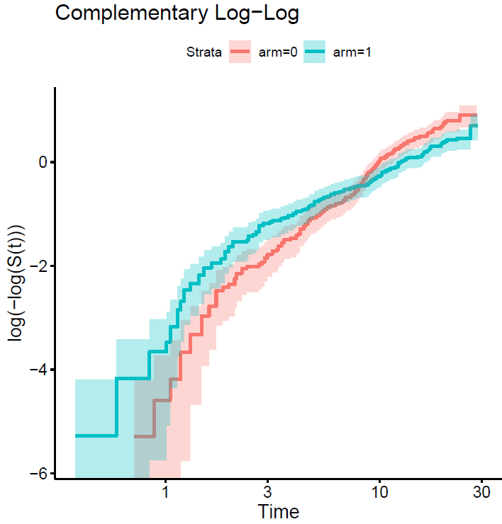
We may know more if you plot the curves on the log relative hazards scale (log(-log(S(t)))).
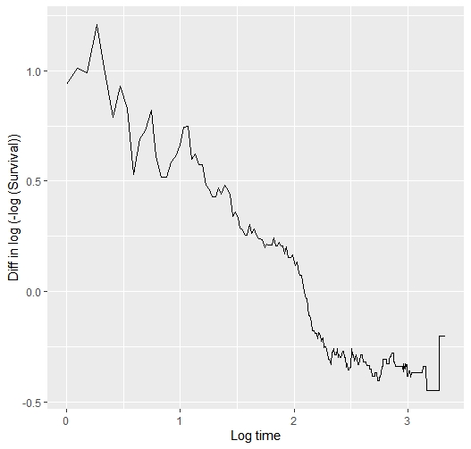
This is the plot…
The point is that each curve has a different morphology, with more or less serious violations of the proportional hazard assumption, and with different fluctuations of the risk. The question is how to model them all with a single pre-specified formulation. The spline-based model picks them up very well but sometimes requires many degrees of freedom to do so. The question is how to pre-specify it in a simple way. You sometimes talk about using Bayesian methods, with priors that favor simple models with few degrees of freedom, but allow more complex models if needed. Perhaps it would make sense to use hyperpriors for the degrees of freedom of the splines, in a hierarchical way…
1 Like
Yes a hierarchical way of thinking is really good. But I’m seeing a fairly linear relationship between log t and the difference in those two curves, so maybe I’m missing your point. In the Cox model we don’t care about the shape of any one of the two curves.
If you can compute the vertical differences between the two curves that would tell is if what I saw is an optical illusion.
1 Like
I have computed the difference between the two arms of the log(-log survival ) vs log(time) plot above. This is the code and the result… so?
survi<-summary(survfit(sur~arm, data = kn061), time=seq(1,28,0.1 ) )
survi$surv=log(-log (survi$surv))
survi$time=log(survi$time)
survi2<-data.frame(strata=survi$strata, time=survi$time, surv=survi$surv)
s0<-survi2[survi2$strata=="arm=1",]
s1<-survi2[survi2$strata=="arm=0",]
survi2$diff= s0$surv- s1$surv
ggplot(data=survi2, aes(x=time, y=diff)) +
        geom_line()
2 Likes
As I guessed, the interaction between log(t) and treatment effect is linear so should be easy and efficient to model treatment with a total of 2 d.f.
1 Like
Ok, so I’m going to fit the model, and then represent its predictions vs Kaplan-Meier. What would the formula be then, arm + arm * log(time)??
1 Like
Yes. There is a vignetted with the R survival package explaining how to do time-dependent covariates. Or use a flexible parametric spline model with a linear restriction for the interaction with log(t).
1 Like
The result is significant when it is done like this. The problem is that I have not managed to obtain the predicted survival rates or the plot to evaluate the goodness of fit because the survival package does not accept this option with tt terms. After searching for a while on the internet I have given up. Does anyone know how to do that?
> coxph(Surv(time,event==1)~arm,data=kn061)
Call:
coxph(formula = Surv(time, event == 1) ~ arm, data = kn061)

       coef exp(coef) se(coef)      z      p
arm -0.2031    0.8162   0.1111 -1.828 0.0675

Likelihood ratio test=3.35  on 1 df, p=0.06713
n= 395, number of events= 330
> coxph(Surv(time,event==1)~arm + tt(arm), tt = function(x, t, ...) x * log(t), data=kn061)
Call:
coxph(formula = Surv(time, event == 1) ~ arm + tt(arm), data = kn061,
    tt = function(x, t, ...) x * log(t))

           coef exp(coef) se(coef)      z        p
arm      0.6665    1.9473   0.2530  2.635 0.008425
tt(arm) -0.4964    0.6087   0.1292 -3.843 0.000122

Likelihood ratio test=18.56  on 2 df, p=9.307e-05
n= 395, number of events= 330
> survfit(cox2)
Error in survfit.coxph(cox2) :
  The survfit function can not process coxph models with a tt term
>I hope that one of the vignettes for survival covers that. It is true that time dependent covariates with a Cox model present complexities at prediction time. If you can get one of the flexible parametric models to fit this 1 d.f. interaction term that would be good. The best review of flexible parametric survival models I’ve seen is here.
Of note is the huge likelihood ratio 2 d.f. \chi^2 statistic, providing strong evidence against the supposition that the two survival curves are superimposable. This is a far cry from what you got assuming PH and a good reason to continue this exercise.
Wow! What a great thread.
Dr. Alberto, did you eventually manage to perform these analyses? I was looking into rstanarm’s survival article, section “6.1 A flexible parametric proportional hazards model”. Do you know if one of these models (mod1_bspline; mod1_mspline2; mod1_mspline2) is compatible with what you called “Bayesian Royston-Parmar model”?
No, I did not try that but would be nice to see examples
1 Like