I have been trying to read through Fedorov et al 2009 so that I can explain it to my clinical colleagues. I understand (and can explain) why dichotomizing a continuous variable leads to a reduction in power (or an increase in required sample size).
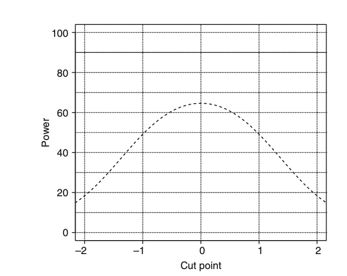
I am having trouble explaining the situation in Figure 2 where they design a hypothesis test with alpha=0.05, mu=0, sigma=1, N=100, and delta=0.29 to give 1-beta=0.9 in the continuous case. I see that this translates in the dichotomous case to the population proportion being 50% and the test for a sample proportion of 38.5%, but I can’t describe why shifting the cutpoint to be +1 or -1 should provide the same decrease in power, since the population proportion would then be 15.8% or 84.2% for corresponding powers of the test.
How are you calculating the power and confidence interval for the proportion? The fact that the estimate of the mean is more efficient (assuming the normal distribution) implies the corresponding test is more powerful.
Alternatively, for a given power, the mean can detect smaller effect sizes than the median test can.
The textbook asymptotic formula \hat{p} \pm Z_\alpha\sqrt{\frac{\hat{p}(1-\hat{p})}{n}} gets less accurate when the proportion is close to 0 or 1, since the variance is closely correlated to the estimate.
There exist variance stabilizing transformations that can widen the range over which the normal approximation is useful [1], but even here, the farther away from the midpoint of the range you get, the less information you have about the proportion. The authors recommend using the arcsine transformation: 2[ arcsin(\sqrt{p}) - arcsin(\sqrt{p_0)} ]. The formula for a confidence interval is in the link to chapter 18 below. They also discuss the log transformation as well.
Addendum: I found the paper and need to read it over. I’ll probably revise this later. What I referred to above is technically correct, but not relevant to the fundamental point of the paper, which is very interesting.
Kulinskaya E., Morgenthaler S., Staudte RG (2008)Meta-Analysis: A Guide to Calibrating and Combining Statistical EvidenceCh 18 Wiley Publishing
I happened to be reading the section on precision for binomial confidence intervals in BBR and was following up on references. The text recommends the Wilson method for a frequentist CI and links to a Wikipedia article. Following up on those citations lead me to a critique of the arcsine transformation I discussed above.
These authors recommend the logistic model for discrete data, or a linear transform for continuous data.
This seems reasonable to me for individual studies, but there might still be a justifiable, educational use of the arcsine transformation in the context of meta-analysis.
The comparison of 38.5% versus 50% has the same power as 62.5% versus 50%. If you observed two groups with proportions experiencing some event of 38.5% and 50%, you could equally consider this two proportions of not experiencing the event (so 62.5% versus 50%). This must have the same power - you have no more information from having reversed the way you consider the proportions. Hence, cutting a continuous variable at plus or minus 1 (with corresponding proportions being the inverse of each other) results in the same power (loss).