RMS Semiparametric Ordinal Longitudinal Model

Johannes_Schwenke · May 17, 2025, 1:01pm

I was thinking about trying to apply the transition model to a cancer trial I’m working on. For every day of follow-up I’ll know whether a patient was at home or in-hospital, or of course deceased. But roughly every 6 weeks the patients also fill a QoL questionnaire (7 level ordinal scale), and I’m wondering whether I can integrate this information.

I’m thinking of a 9 levels ordinal scale, 1 being the best quality of life, …, 7 being the worst QoL, 8 being hospitalized, and 9 as the absorbing state death. I’m wondering if it’s possible to handle the unknown QoL between two measurements. I know that if a patient is not deceased and not in hospital, so she/he must have state 1:7. But given that this will be the case for >95% days a patients is not hospitalized handling this seems unfeasible? I wouldn’t even know where to start. I definitely don’t think I could justify carrying the last value forward. Has there been done any work for this kind of problem?

f2harrell · May 17, 2025, 2:34pm

A great question. For frequentist models, rms::orm handles censoring, and for Bayesian models there’s rmsb::blrm with examples at RMSb. Under the proportional odds assumption, you can treat partial data as interval, left, or right censored. Carry forward is another option but assumes patients are very stable. Multiple imputation is another option, but that’s more for the case where you potentially have lots of QoL assessments with many randomly missing.

Johannes_Schwenke · May 17, 2025, 3:59pm

So great! This example is exactly what I needed : rmsb Package Examples Using rstan.

Johannes_Schwenke · May 17, 2025, 5:57pm

Is it already possible to use such a model with censored data and thus censored previous states to get state occupancy probabilities?
I’m not sure how I have to specify pvarname, given that’s it’s a matrix and not directly found in the data. pvarname = “Ocens(yprev.a, yprev.b)” ofc returns “not found in data”. I’m also still quite confused general what’s going on under the hood if we use an interval censored predictor.
Thanks!

model <-
    blrm(
      formula = Ocens(y.a, y.b) ~ Ocens(yprev.a, yprev.b) + rcs(time, 6) * tx,
      data = data,
      ppo = ~ time,
      refresh = 5,
      iter = 2000,
      chains = 4,
      method = "sampling"
  )

sop_tx1 <- soprobMarkovOrdm(
  model,
  data = list(tx = 1, yprev.a = 3, yprev.b = 3),
  times = 1:26,
  ylevels = 1:9,
  absorb = 9,
  tvarname = "week",
  pvarname = ????
)

f2harrell · May 17, 2025, 7:24pm

You’ve hit one roadblock with this approach. Ocens is only for the left hand side of the model. We do have a problem thinking about conditioning on something that is only partially known. Though we don’t do this for the left hand side of the model, we may need to use a carry-forward for the previous value of Y, or multiple imputation.

Johannes_Schwenke · May 20, 2025, 7:19am

Sorry if I’m asking too many questions. I was wondering: Is this model also suited for recurrent events, of which there could be multiples in a single day?

Let’s say we want to test potentially less effective, but also less toxic drug against SoC. We want to test for difference in toxicity while taking into account mortality. Good markers for toxicity would be blood transfusions. Overall, transfusions will be rare, but if you’re unlucky you might need quite a few in a single day.

I imagine we’d then code individual days something like this.

0 - 0 transfusions
1 - 1 transfusion
…
6 - 6 transfusions
7 - death

A patient might then have states like this

000 … 0200 … 00067

We could easily calculate the expected number of days without any transfusion but I think many clinicians would prefer an estimand which is more closely related to the rate / count of the transfusions. I probably need to think more carefully about the questions which we want to answer in this case.

I’m probably just being thick? Would be the expected number of transfusions just be
1 * sum of SOPs across state 1 + 2 * sum of SOPs across state 2 + … + 6 * sum of SOPs across state 6?

For a frequentist framework, others have recommended quasi-poisson, or for a bayesian approach shared frailty models (e.g., poisson, weibull, with shared frailty as a gamma), but the assumptions are quite strong.

f2harrell · May 20, 2025, 11:09am

I like your thinking, i.e., you are starting with getting for each day the SOP of # transfusions = i for some i, and summing these SOPs gives you the expected number of days with i transfusions. Then sum those over i. Maybe easier to think about: separately for each day estimate the expected number of transfusions by summing all of that day’s SOPs over i, then sum over days.

Poisson would assume constant transfusion rate over time, and would not reveal time trends.

Johannes_Schwenke · May 26, 2025, 7:31pm

Edit: It was of course human error. Yprev was not formatted as a factor. After fixing this, the results are much better! Though, I now have to collapse state 3 and 4, because state 3 has very few observations (35) and this results in extraordinary numbers of divergent transitions. Is there any guidance how many observations for a non-absorbing state are needed?

I’ve been experimenting a bit more with the ordinal longitudinal model but am struggling with very bad predictions of SOPs.

I have some historical data (which I, unfortunately, cannot share) of 271 patients, which were all followed for 182 days or until death.

I have coded their levels as follows:

1 - At home;
2 - planned hospitalization;
3 - emergency room visit;
4 - emergency hospitalization;
5 - death

Everyone is at home (state = 1) at baseline. Cumulative incidence of death is around 15%.

Empirical SOPs:

Empirical Transition Probabilities:

Correlation between days doesn’t seem to be constant over the follow-up period, so I thought it a good idea to interact yprev with time.

Correlation Plot:

I fit a model without covariates (of course using a dataset which does not carry death forward):

model <-
    blrm(
      formula = y ~ yprev * rcs(day, 5),
      data = data_ordinal,
      ppo = ~ day,
      cppo = function(y) y,
      refresh = 5,
      iter = 2000,
      chains = 4,
      method = "sampling"
  )

Model Summary

Bayesian Constrained Partial Proportional Odds Ordinal Logistic Model

Dirichlet Priors With Concentration Parameter 0.392 for Intercepts

blrm(formula = y ~ yprev * rcs(day, 5), ppo = ~day, cppo = function(y) y, 
    data = data_ordinal, iter = 2000, chains = 4, refresh = 5, 
    method = "sampling")


Frequencies of Responses

    1     2     3     4     5 
41770  1114    35  1760    40 

                  Mixed Calibration/             Discrimination               Rank Discrim.    
              Discrimination Indexes                    Indexes                     Indexes    
  Obs44719    B 0.023 [0.022, 0.023]    g  1.305 [1.217, 1.383]    C   0.944 [0.942, 0.944]    
 Draws4000                              gp 0.097 [0.095, 0.098]    Dxy 0.887 [0.885, 0.889]    
  Chains 4                              EV 0.644 [0.633, 0.656]                                
Time880.1s                              v    4.115 [3.86, 4.35]                                
  p      9                              vp 0.039 [0.039, 0.039]                                

               Mean Beta Median Beta S.E.   Lower    Upper    Pr(Beta>0)
y>=2            -7.6776   -7.6759    0.2379  -8.1417  -7.2099 0.0000    
y>=3            -9.6974   -9.6999    0.2548 -10.2053  -9.2122 0.0000    
y>=4            -9.9413   -9.9414    0.2705 -10.4456  -9.3843 0.0000    
y>=5           -17.4511  -17.4555    0.3725 -18.1713 -16.7255 0.0000    
yprev            3.7530    3.7549    0.1526   3.4375   4.0354 1.0000    
day              0.0309    0.0309    0.0085   0.0137   0.0471 1.0000    
day'            -0.2385   -0.2389    0.0562  -0.3435  -0.1244 0.0000    
day''            0.6166    0.6154    0.1647   0.3073   0.9472 1.0000    
day'''          -0.5668   -0.5680    0.2095  -0.9585  -0.1346 0.0043    
yprev * day     -0.0209   -0.0209    0.0053  -0.0310  -0.0104 0.0000    
yprev * day'     0.1349    0.1347    0.0344   0.0667   0.1991 1.0000    
yprev * day''   -0.3680   -0.3683    0.1000  -0.5555  -0.1692 0.0000    
yprev * day'''   0.3808    0.3837    0.1255   0.1356   0.6272 0.9990    
day x f(y)       0.0009    0.0009    0.0004   0.0001   0.0017 0.9842    
               Symmetry
y>=2           1.01    
y>=3           1.01    
y>=4           1.02    
y>=5           1.01    
yprev          0.97    
day            1.01    
day'           1.01    
day''          0.98    
day'''         1.00    
yprev * day    1.01    
yprev * day'   0.97    
yprev * day''  1.01    
yprev * day''' 0.99    
day x f(y)     0.99

Model diagnostics are fine.

Given that we use no covariates and everyone in our dataset starts with state = 1, the conditional SOPs should equal the marginal SOPs unless I’m mistaken.

However, when I compare the model derived SOPs with the empirical ones, they are widly different, especially for state 4 (death).

Calculating SOPs

sop <- soprobMarkovOrdm(
  model,
  data = list(yprev = 1),
  times = 1:182,
  ylevels = 1:5,
  absorb = 5,
  tvarname = "day",
  pvarname = "yprev"
)

sop <- as.data.table(sop)

# Rename columns
setnames(sop,
         old = c("V1", "V2", "V3", "value"),
         new = c("draw", "day", "state", "sop"))

sop_placebo$day <- as.integer(sop$day)
sop_placebo$state <- as.factor(sop$state)

Empirical SOP vs Model derived SOP

I’m a bit lost as to what to trouble shoot. I checked the datasets multiple times for errors.
Is it possible that the data just isn’t suited for the transition model? Is this obvious from the empirical plots? I’m not yet comfortable in interpreting them. Many thanks.

Johannes_Schwenke · June 23, 2025, 2:40pm

I have a question regarding relaxing the PO assumption.

Let’s say we want to relax the PO assumption for time for all levels of Y, as is done in many of FH’s examples AND we also want to relax the PO assumption for one level of Y for the treatment indicator.

For example, in a setting with high mortality, we examine an intervention, which should improve patients QoL, but is unlikely to affect mortality. The estimand could be something like : “Difference in mean days spent with good or better QoL”.

If the intervention strongly improves QoL, but not mortality, I assume this would make the model predict a difference in the cumulative incidence of death, even though there is none, and give incorrect estimates of days spent with x QoL.

However, fully relaxing the PO assumption for tx seems unreasonable, because a PO effect of tx on QoL is very plausible.

Something inbetween

blrm(
      formula = Ocens(y.a, y.b)  ~ tx * rcs(day, 4) + yprev * rcs(gap, 3),
      data = df,
      ppo = ~ day * tx,
      cppo = function(y) y,
      refresh = 5,
      iter = 2000,
      chains = 4,
      method = "sampling"
  )

and

blrm(
      formula = Ocens(y.a, y.b)  ~ tx * rcs(day, 4) + yprev * rcs(gap, 3),
      data = df,
      ppo = ~ day,
      cppo = function(y) y,
      refresh = 5,
      iter = 2000,
      chains = 4,
      method = "sampling"
  )

Initially I thought about using function(y) y == 8, so PPO only affects death, but I don’t think that would work, because we need to relax PO assumption over day for levels 1-7.

I assume it’s possible to put priors on the dissimilarity of the treatment effect, but as I’m quite new to all of this, I don’t really know how. Ofc I might have also misunderstood some things. Any insights would ab appreciated!

f2harrell · June 24, 2025, 6:37am

For a frequentist solution to this you may be able to use the VGAM or ordinal packages. But to do this efficiently for a high number of quality of life levels you’ll need to wait until I enhance rms::orm and rmsb::blrm to allow cppo to contain a matrix of transformations. Even then, we need to make sure that the planned enhancements cover the situation adequately. I was going to implement cppo as a user-specified transformation matrix where in your case the first column may be y (to allow a smooth linear departure from PO) and the second column may be y==8 to allow a special effect on death. I wonder if this handles time adequately without giving too much overfitting with respect to treatment.

Johannes_Schwenke · June 24, 2025, 8:36am

Thanks. Looking very much forward to the updates.

Johannes_Schwenke · July 2, 2025, 11:19am

Other day, other question regarding the transition model. I’m trying to incorporate partial information with Ocens().

I’m interested in a scenario, where
A) we know the baseline value (inital yprev) for everyone,
B) we know the day of the absorbing state (if it happened) for everyone, and
C) all other states in between are missing at random with a high percentage 80-90%.

I carry the last observed value forward as yprev, include a gap time to the last definitely known value, and interact it with yprev.

What the dataset looks like

blrm(
      formula = Ocens(y.a, y.b) ~ yprev * gap + age + rcs(day, 4) + tx,
      ppo = ~day,
      cppo = function(y) y,
      data = df_censored,
      refresh = 5,
      iter = 2000,
      chains = 4,
      method = "sampling"
    )

I find that when we only observe a couple of values in between per patient, e.g., about 3 non-absorbing states obs per patient, the marginalized cumulative incidence of death is a crass overestimate of the empirical SOPs.

I would have expected the estimates for the non-absorbing states to be very poor, but not for the absorbing state. If we observe about 50% of the non-censored states, the estimates are fine.

Is the issue just a hard limitation when we have so much partial information for non-absorbing states only? Or is there a mistake in my approach in general?

Example for the simulated VIOLET data with 90% censoring.

Left: empirical SOPs before we randomly remove non-absorbing states observations.
Right: model-derived marginalized SOPs from censored dataset.

Code to reproduce

# Sorry about the mix between tidyverse and data.table()

# Load packages

library(tidyverse)
library(data.table)
library(Hmisc)
library(ggplot2)
library(rmsb)
library(furrr)

set.seed(123)

fit <- TRUE #set to true if you want to fit the model
generate_SOPS <- TRUE


# Load simulated VIOLET data from Hmisc data repository
Hmisc::getHdata("simlongord")

# Only use 500 random participants
ids <- sample(unique(simlongord$id), 300, replace = FALSE)
df <- filter(simlongord, id %in% ids)

setDT(df)

# Select required columns
df <-
  df |>
  select(id, tx, age, day = time, y, yprev, gap)


# Replace IDs with numbers
df$id <- as.integer(as.factor(df$id))

# Recode data types
df$tx <- factor(df$tx)
df$age <- as.integer(df$age)
df$day <- as.integer(df$day)
df$yprev <- as.factor(df$yprev) |> fct_rev() |> as.integer() |> as.factor()
df$y <- as.ordered(df$y) |> fct_rev() |> as.integer() |> as.factor()
df$gap <- as.integer(df$gap)


death_dates <-
  filter(df, y == 4) |>
  select(id, ddeath = day)

df <- left_join(df, death_dates, by = "id")

# create a version of the dataset where we carry death forward
df_state_4 <-
  df |>
  mutate(y = as.integer(y), yprev = as.integer(yprev)) |>
  filter(y == 4) |>
  group_by(id) |>
  complete(day = ddeath:28, fill = list(y = 4L, yprev = 4L, gap = 1)) |>
  arrange(id, day) |>
  fill(everything())

df_state_1_to_3 <-
  df |>
  mutate(y = as.integer(y), yprev = as.integer(yprev)) |>
  filter(y != 4) |>
  arrange(id, day)

df_forward <-
  bind_rows(df_state_1_to_3, df_state_4) |>
  mutate(y = as.ordered(y), yprev = as.factor(yprev)) |>
  arrange(id, day)

# empirical SOPs
df_forward |>
  ggplot(aes(x = day, fill = factor(y))) +
  geom_bar(position = "fill") +
  scale_fill_brewer(palette = "Dark2") +
  facet_wrap(~tx)


# Remove 85% of the observations between baseline and death
first_rows <- df |>
  group_by(id) |>
  arrange(id, day) |>
  slice_head(n = 1)

death_rows <- df |>
  filter(y == '4')

sample_rows <- df |>
  anti_join(death_rows) |>
  ungroup() |>
  slice_sample(prop = 0.10) |>
  arrange(id, day)

# recompute yprev and add gap tiome between measurements
baseline <- first_rows |>
  mutate(
    y = yprev,
    day = 0
  ) |>
  select(-yprev)

follow_up <- sample_rows |>
  bind_rows(death_rows) |>
  select(-yprev) |>
  bind_rows(baseline) |>
  arrange(id, day)

follow_up <- follow_up |>
  group_by(id) |>
  mutate(
    yprev = case_when(
      TRUE ~ lag(y, n = 1, order_by = day)
    ),
    yprev = factor(yprev, levels = 1:3, ordered = FALSE), #death = 8 doesn't exist in yprev
    dayprev = case_when(
      TRUE ~ lag(day, n = 1, order_by = day)
    ),
    gap = day - dayprev
  ) |>
  slice(-1) |> #remove baseline without prior state
  ungroup()

# create censored data set
df_censored <- follow_up |>
  select(-y, -yprev, -day, -dayprev, -gap) |>
  distinct() |>
  mutate(day = list(1:28)) |>
  unnest(day) |>
  left_join(follow_up |> select(id, day, y, yprev), by = c("id", "day")) |>
  mutate(
    yprev = as.numeric(as.character(yprev)),
    y = as.numeric(as.character(y))
  ) |>
  group_by(id) |>
  fill(yprev, .direction = "up") |>
  mutate(
    yprev = case_when(
      is.na(yprev) ~ lag(y, n = 1, order_by = day),
      TRUE ~ yprev
    ),
    y.a = case_when(
      !is.na(y) ~ y,
      TRUE ~ 1
    ),
    y.b = case_when(
      !is.na(y) ~ y,
      TRUE ~ 3
    )
  ) |>
  fill(yprev, .direction = "down") |>
  mutate(gap_group = cumsum(lag(!is.na(y), default = FALSE))) |>
  group_by(id, gap_group) |>
  mutate(gap = row_number()) |>
  ungroup() |>
  filter(yprev != 4) |> #remove death carried forward
  select(-gap_group) |>
  mutate(
    yprev = factor(yprev),
    tx = factor(tx)
  )

# model fitting
options(mc.cores = 8)

set.seed(777)

Sys.setenv(RSTUDIO = 1)
if (fit) {
  model <-
    blrm(
      formula = Ocens(y.a, y.b) ~ yprev * gap + age + rcs(day, 4) + tx,
      ppo = ~day,
      cppo = function(y) y,
      data = df_censored,
      refresh = 5,
      iter = 2000,
      chains = 4,
      method = "sampling"
    )

  # Save model to an RDS file
  saveRDS(model, "./fitted_models/model_censoring.rds")
}
Sys.setenv(RSTUDIO = 0)

# get marginalized SOPs
baseline_df <- filter(df_censored, day == 1) |> as.data.table()


write_SOP <- function(i, tx, baseline_df) {
  row <- baseline_df[i]

  sops <-
    soprobMarkovOrdm(
      model,
      data = list(tx = tx, age = row$age, yprev = row$yprev, gap = 1),
      times = 1:28,
      ylevels = 1:4,
      absorb = 4,
      tvarname = "day",
      pvarname = "yprev"
    )

  # Because of the size of the data, only use the first 500 MCMC draws
  sops <- sops[1:500, , ]

  sops <- as.data.table(sops)

  # Rename columns
  setnames(
    sops,
    old = c("V1", "V2", "V3", "value"),
    new = c("draw", "day", "state", "sop")
  )

  sops$day <- as.integer(sops$day)
  sops$state <- as.factor(sops$state)
  sops$tx <- tx
  sops$i <- i

  folder <- glue::glue("marginalized_sop_{tx}/msop_{i}.parquet")

  arrow::write_parquet(
    x = sops,
    sink = folder
  )
}
future::plan(multisession, workers = 6)

# Generate marginalized SOPs
# Placebo
if (generate_SOPS) {
  furrr::future_walk(
    1:nrow(baseline_df),
    \(x) write_SOP(x, 0, baseline_df),
    .progress = TRUE,
    .options = furrr_options(seed = TRUE)
  )
}

# Treatment
if (generate_SOPS) {
  furrr::future_walk(
    1:nrow(baseline_df),
    \(x) write_SOP(x, 1, baseline_df),
    .progress = TRUE,
    .options = furrr_options(seed = TRUE)
  )
}

# Read maginalized SOPs

# Get list of all files
files <- fs::dir_ls("./marginalized_sop_0/", glob = "*.parquet")

# Read in each parquet file as a data.frame and merge into a data.table
placebo_df <- map(files, \(x) arrow::read_parquet(x), .progress = TRUE) |>
  rbindlist()

# Average SOPs over covariate settings -- for each state, day, and MCMC draw
placebo_df <- placebo_df[, .(sop = mean(sop)), by = .(state, day, draw, tx)]
placebo_df[, state := as.factor(state)]

# Get list of all files
files <- fs::dir_ls("./marginalized_sop_1/", glob = "*.parquet")

# Read in each parquet file as a data.frame and merge into a data.table
tx_df <- map(files, \(x) arrow::read_parquet(x), .progress = TRUE) |>
  rbindlist()

# Average SOPs over covariate settings -- for each state, day, and MCMC draw
tx_df <- tx_df[, .(sop = mean(sop)), by = .(state, day, draw, tx)]
tx_df[, state := as.factor(state)]

sop_df <-
  bind_rows(placebo_df, tx_df) |>
  mutate(tx = as.factor(tx))


sop_df |>
  group_by(day, state, tx) |>
  summarise(sop = median(sop)) |>
  group_by(day, tx) |>
  mutate(sop = sop / sum(sop)) |>
  ungroup() |>
  ggplot(aes(x = day, y = sop, fill = state)) +
  geom_col() +
  scale_fill_brewer(palette = "Dark2") +
  facet_wrap(~tx) +
  labs(x = "week")

f2harrell · July 2, 2025, 11:29am

I’m glad you are investigating this. It is very much an open area for research. Would you mind commenting on the simulations I’ve done in one of the documents here, i.e., are there any similarities between what the two of us observed? It would also be adding SOP plots where the interaction is excluded and where both the interaction and the gap times are excluded from the model, and to also compare with a multiple imputation approach.

Johannes_Schwenke · July 2, 2025, 12:28pm

Thanks. The links doesn’t seem to work for me.

I went through this analysis of yours, which is different insofar that it doesn’t concern absorbing states. I also looked at this. Here the section 10 on response-dependent sampling is somewhat similar, but it’s different as observations after having reached state “discharged” are still quite frequent (every 3 days) and mostly missing in those patient who will not move to the absorbing state death (?). Also, documents do not make use of the Ocens() function.

Regarding the multiple imputation : what would be your approach to imputing the missing observations to populate to yprev with / what is reasonable? Until recently i would simply have used MICE with id as a clustering variable, but that would then assume a compound symmetry, would it not, which might not be ideal? And would you impute y to populate yprev and then use Ocens() again for Y, or actually used to imputed values for Y as well?

I shall exclude the interaction, gap times, and do more tests with imputation, and report back.

f2harrell · July 2, 2025, 6:14pm

I think the link is fixed now but I think you already found the more particular links. Regarding the imputation strategy, I’ve been tempted to use Stata’s within-person backwards/forwards approach, one piece of which might be thought of as next observation carried backwards, and letting that one override last value carried forward if the gap is smaller. There’s more to the algorithm. Then there is the more traditional imputation you alluded to; for that I don’t think getting the correlation pattern right is a huge problem and using a working independence model might possibly even work.

For either approach one of many open question is whether to impute all the Y values, then form yprev from them, or to just impute yprev and use interval censoring for handling Y.

Johannes_Schwenke · August 18, 2025, 12:29pm

I’m trying to develop a better understanding and intuition for the transition model and was wondering how you choose to model the correlation structure of yprev and time. I’m also having some concerns regarding error rates.

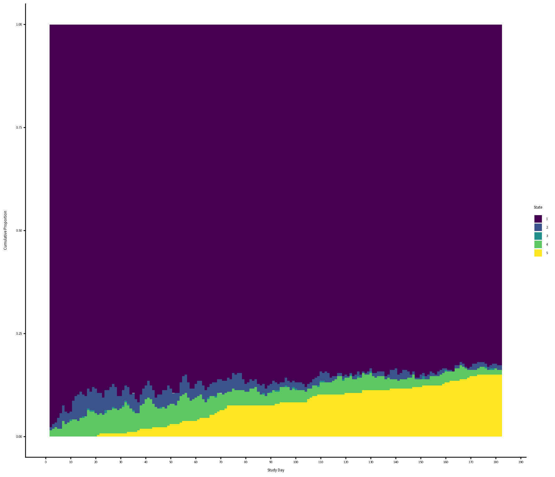
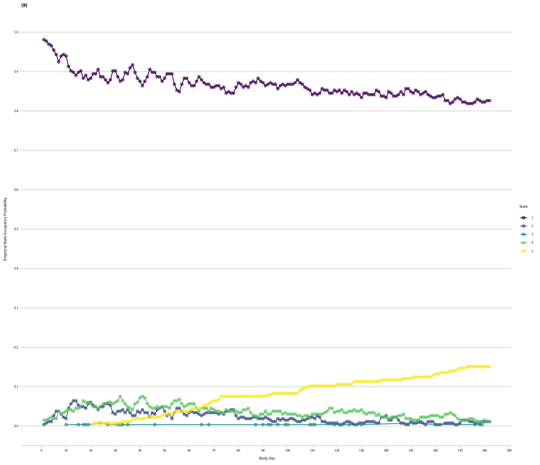
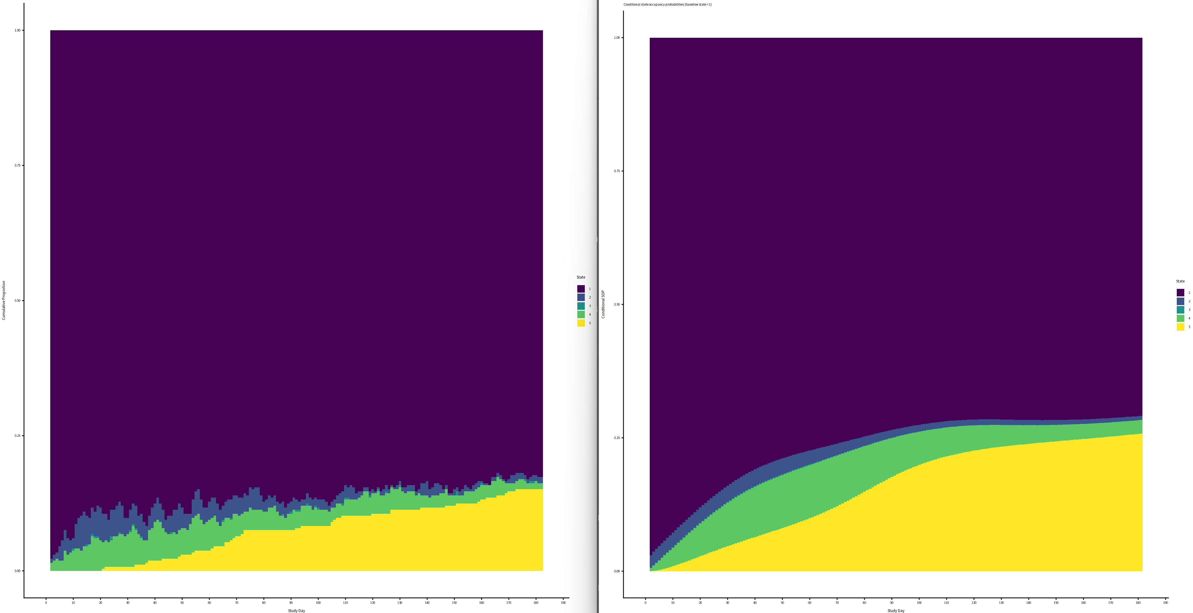
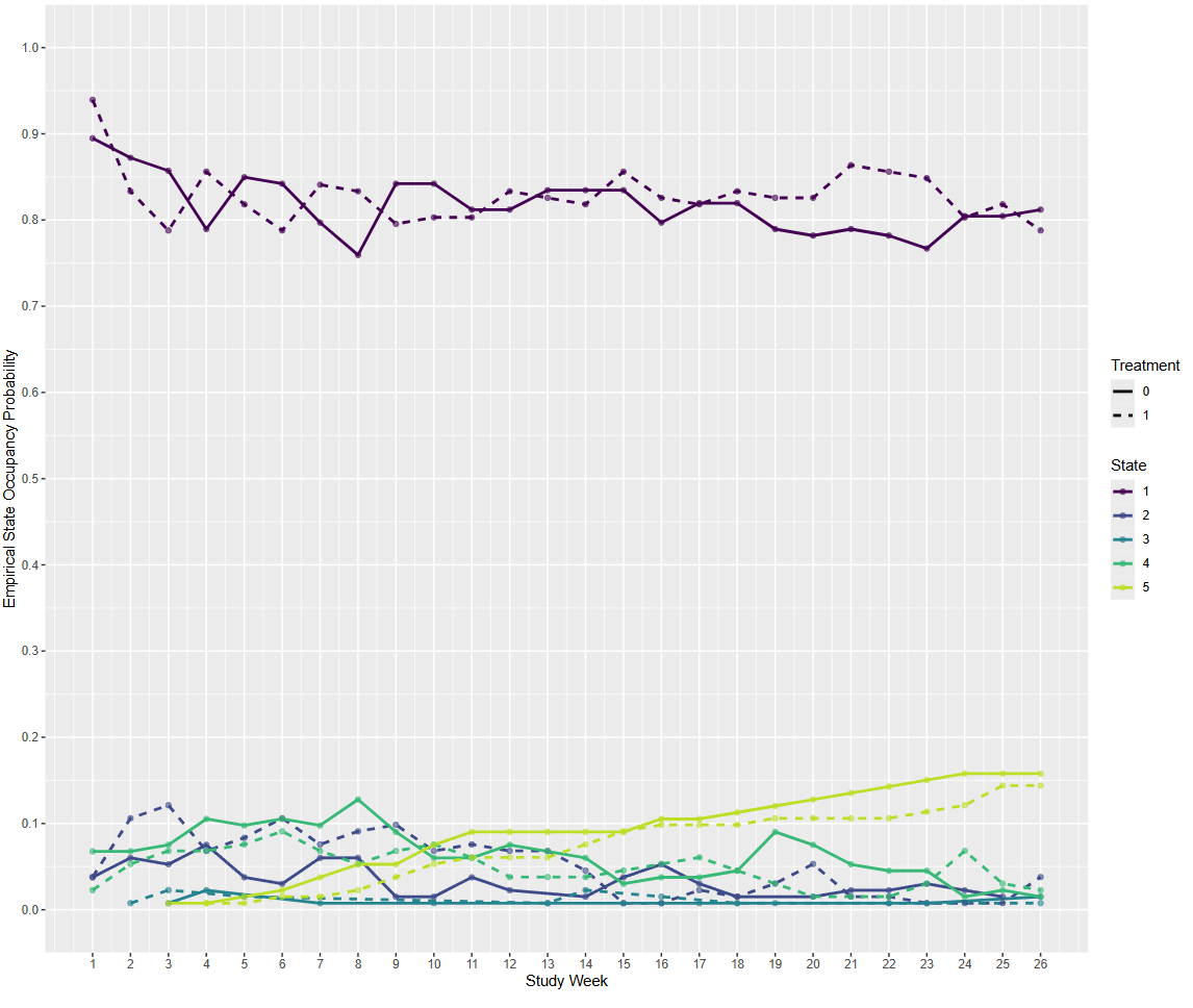
For context, I’m using a historical dataset of Stage IV cancer patients who were not in an RCT: 260 patients followed for 26 weeks. I have weekly data on whether they are at home [1], in hospital for planned treatment [2], visited the ER [3], were in hospital for an emergency [4], or dead [5]. I had to collapse state [3] and [4], because [3] is very rare. Patients spent most of their time in state 1, see empirical SOPs.

Empirical SOPs

I’ve randomly divided the patients into ‘treated’ and ‘control’ to mimic a null RCT.

Questions about modelling time and yprev

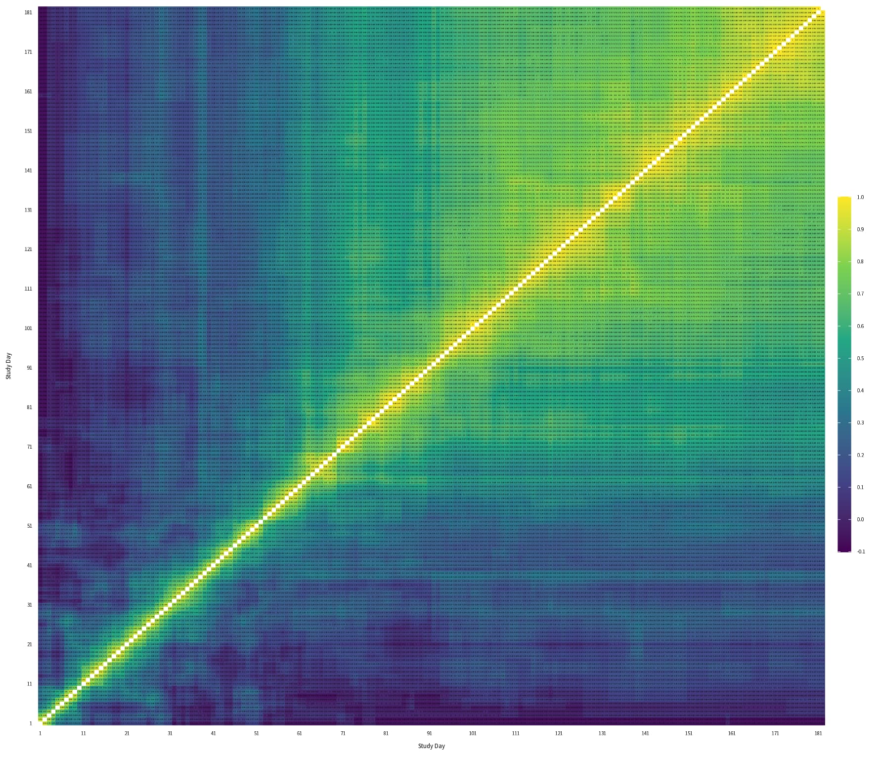
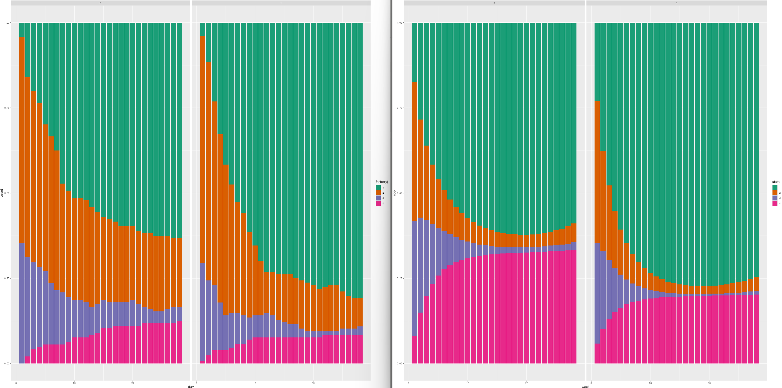
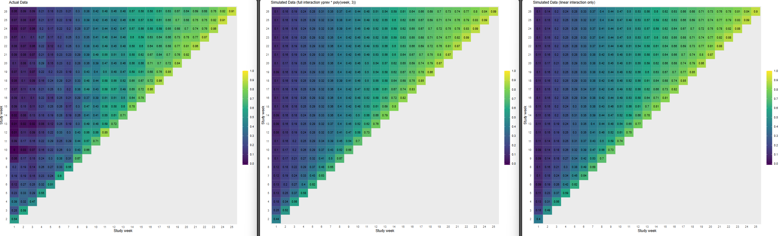
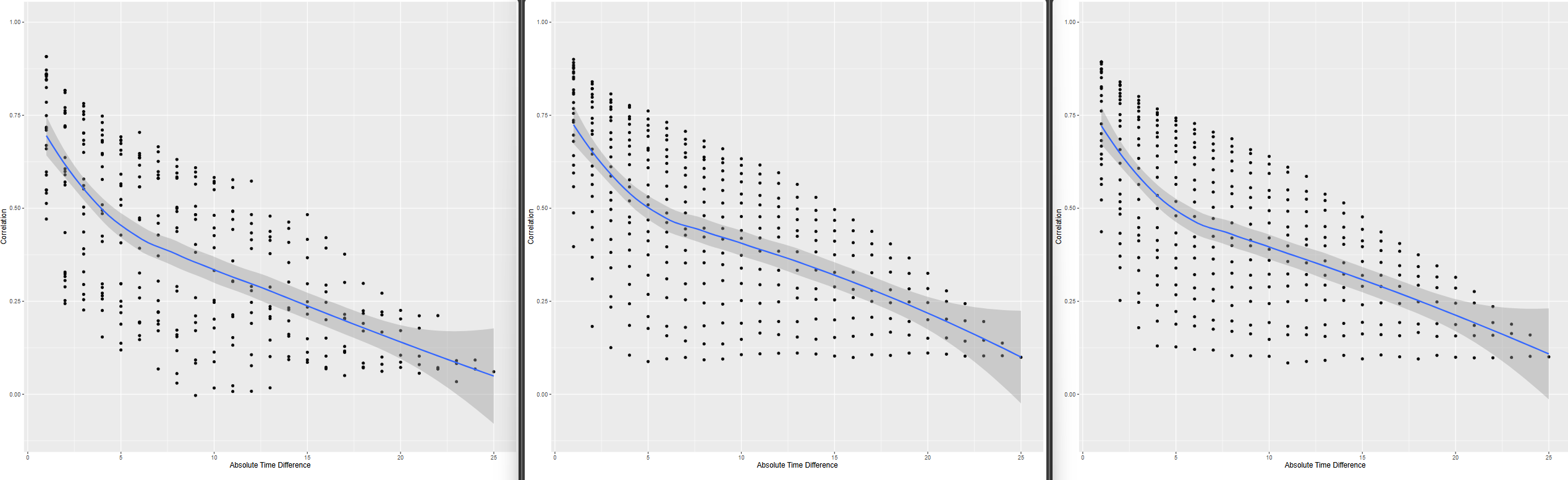
Following your paper, and chapter 22 from RMS, I constructed the empirical correlation matrix and variogram and compared those to plots made from simulated data, based on three different models fit to the original data: 1) no interaction between y and yprev, 2) linear interaction between y and yprev, 3) and full interaction between y and yprev. (No interaction not shown on plots, slightly worse fit than linear interaction)

Models used for simulated data

# I modelled time with a 3rd degree polynomial instead of splines because I found it easier to reconstruct the linear predictor for the simordmarkov function and took the median of the parameter estimates instead of all draws.

model_full_int <-
      blrm(
        formula = y  ~ tx + pol(week, 3) * yprev + ecog_fstcnt + diagnosis + age + gender + albumin + c_reactive_protein,
        data = df,
        ppo = ~ week,
        cppo = function(y) y,
        iter = 2000,
        chains = 4
    )

model_lin_int <-
      blrm(
        formula = y  ~ tx + pol(week, 3) + yprev + yprev %ia% week + ecog_fstcnt + diagnosis + age + gender + albumin + c_reactive_protein,
        data = df,
        ppo = ~ week,
        cppo = function(y) y,
        iter = 2000,
        chains = 4
    )

model_no_int <-
      blrm(
        formula = y  ~ tx + pol(week, 3) + yprev + ecog_fstcnt + diagnosis + age + gender + albumin + c_reactive_protein,
        data = df,
        ppo = ~ week,
        cppo = function(y) y,
        iter = 2000,
        chains = 4
    )

Empirical | Full Interaction | Linear Interaction

Mean absolute difference between empirical and model based correlation coefficients as a function of week:

model	1	2	3	4	5	6	7	8	9	10	11	12	13	14	15	16	17	18	19	20	21	22	23	24	25	26
full_int	0.05	0.06	0.08	0.06	0.09	0.07	0.12	0.08	0.04	0.06	0.03	0.06	0.09	0.05	0.05	0.06	0.05	0.05	0.05	0.06	0.05	0.05	0.05	0.07	0.05	0.05
lin_int	0.06	0.06	0.09	0.06	0.10	0.08	0.14	0.10	0.05	0.08	0.04	0.06	0.10	0.06	0.05	0.06	0.05	0.05	0.05	0.07	0.06	0.06	0.05	0.07	0.06	0.06
no_int	0.06	0.06	0.11	0.10	0.14	0.12	0.17	0.12	0.07	0.10	0.06	0.08	0.11	0.07	0.05	0.06	0.05	0.05	0.06	0.07	0.06	0.07	0.06	0.08	0.07	0.07

When I compare the empirical correlation matrix and variogram to the simulated ones, none of them look particularly great compared to the fit of the simulated data for the VIOLET trial.
I lack experience, so I’m wondering if this approximates the empirical structure well enough? Is there any guidance on what’s not good enough? The full interaction seems to be closest to the correlation structure, but I’d be tempted to use the linear interaction only, for parsimony.
I’m also a bit confused if not getting the correlation structure approx. right affects the type I assertion rate? I would assume it does if I choose an estimand based on SOPs and not just the beta for treatment, like time at home?

Type I Assertion Rate Concerns

I ran 1200 simulations where I randomly divided the dataset into ‘control’ and ‘intervention’ and fitted the following three frequentist models:`

m1 <- vglm(
         ordered(y) ~ tx + rcs(time, 4) + yprev,
         cumulative(reverse = TRUE, parallel = FALSE ~ rcs(time, 4)),
         data = data)
         
m2 <- vglm(
         ordered(y) ~ tx + rcs(time, 4) + yprev + time %ia% yprev,
         cumulative(reverse = TRUE, parallel = FALSE ~ rcs(time, 4)),
         data = data)
         
m3 <- vglm(
         ordered(y) ~ tx + rcs(time, 4) + yprev + ypprev,
         cumulative(reverse = TRUE, parallel = FALSE ~ rcs(time, 4)),
         data = data_yppre

The type I error rate is > 0.05 when choosing alpha of 0.05 as a cut-off:

Simulation	Type I Error (MCSE)
Non-linear	0.068 (0.008)
Linear	0.068 (0.008)
Second-order	0.072 (0.008)

I also ran a simulation using bootstrapping whole patients and increasing the sample size to 500, and the error/assertion rate was even higher, ~ 10%.

I honestly don’t understand why I’m seeing this error inflation. This seems like a problem, but maybe my approach is flawed? Why could I be observing error rates > 0.05?

When using blrm() with default priors, linear constraint on ppo for time, and P(any benefit) > 0.95 for making an assertion of benefit, the error rates are very similar compared to the frequentist models:

Model	Point Estimate	Rejection Rate	Bias	Coverage	Empirical SE	Model SE
no_int	0.002 (0.003)	0.069 (0.007)	0.002 (0.003)	0.929 (0.007)	0.105 (0.012)	0.095 (0.000)
linear_int	0.002 (0.003)	0.072 (0.007)	0.002 (0.003)	0.932 (0.007)	0.105 (0.013)	0.095 (0.000)
full_int	0.002 (0.003)	0.071 (0.007)	0.002 (0.003)	0.932 (0.007)	0.106 (0.013)	0.095 (0.000)
no_int_cluster	0.001 (0.004)	0.041 (0.006)	0.001 (0.004)	0.957 (0.006)	0.128 (0.013)	0.133 (0.000)

The only thing that made a difference, was adding + cluster(id), wich reduced the error / assertion rate. The mean SD of the random effect was about 0.6 across the simulations. Does this mean that the increased error rates are because the first-order (and second-order) markov assumptions do not hold, and the random effect accounts for that?

Sorry for the long post. Any insights would be very much appreciated.

Edit:

To add to my confusion:

When taking simulated data (dataset of 200k patients) without an interaction between time and yprev, i.e., based on this model:

# states three and four were already collapsed during model fitting
vm <- vglm(
  ordered(y) ~ tx + week + I(week^2) + I(week^3) + yprev + ecog_fstcnt + diagnosis,
  cumulative(reverse = TRUE, parallel = FALSE ~ week + I(week^2) + week + I(week^3)),
  data = df
  )

And then running 1000 simulation on this data with n = 250 and using this vglm model, which correctly models time and yprev:

m <- vglm(
  ordered(y) ~ tx + poly(time, 3) + yprev,
  cumulative(reverse = TRUE, parallel = FALSE ~ poly(time, 3)),
  data = data)

I still get inflated Type I error rates of .068 (0.008).

When I increase the sample size per iteration to 1000, the error rate goes down to 0.055 (0.007). Why would it be a matter of sample size? If I had left in state 3 in the simulated data, that might have created problems, because it was so rare, but I already collapsed states 3 and 4 before fitting the model for the simulation, so that can’t be the problem.

f2harrell · August 20, 2025, 2:56pm

As an aside, “error rate” though commonly used to describe \alpha has nothing to do with making errors, i.e., with conclusions being incorrect. I call this type I assertion probability \alpha.

\alpha can be increased by the types of lacks of fit you examined plus non-PO in tx.

You are doing a wonderful job in studying various model fits and doing simulations. I think the 3 types of fits you studied are close calls. I’m not seeing why you said that the correlation structure fit looks worse than with VIOLET. I would make the choices more on the basis of AIC. Get AIC of simplest model, then add interaction between previous state and time, then go back to the simplest model and add a lag-2 to see if a second order Markov fits better than a 1st order. You have to be careful because a 2nd order model has fewer observations than a 1st order one, so work to ensure comparability.

To the best model add random effects and look at their SD.

Having a sparse Y category doesn’t matter when PO holds. It does matter when you relax PO. Try to make sure that the relaxation of PO does not add k-2 parameters to the model where k is the number of Y categories. A constrained partial PO model is what you really want. For example if the highest category is death you might allow a baseline covariate to have a special effect on death but no other special effects.

Once you get a model you think you like, do the variogram-like plots on this model, against the raw data correlation structure.

Johannes_Schwenke · August 20, 2025, 8:38pm

Thanks for your kind words.

I mainly said so because the mean absolute difference of the correlation coefficients as a function of the time unit were much smaller here, pretty much all 0.02, whereas for my dataset it’s >> 0.05 most often.

Yes, I’ve done some comparisons, which lead me to two questions:

A) are you aware of frequentist packages that allow one to fit constrained non-PO terms ? With vglm I’m only able to fit a non-parallel term as complex as in the model formula, i.e., if I use rcs(time, 4) in the formula, I also have to use it for the non-parallel term, which adds far too much complexity. With the ordinal package i can at least model the linear part of time only as non-parallel, but I don’t think constrained is possible either (?). Or maybe I’m missing something in the documentation? I’m personally more than happy with rmsb, but that’s not everyone…

B) Am I understanding correctly that Hmisc functions like soprobMarkovord only support first-order models?

Thanks!

Edit: Here are some comparison based on AIC I’ve done, all with the ordinal package. All models are fitted on the same data (week 1 removed).

Model code

# PO for time
fit_first_po <- clm(
  formula = y ~ rcs(week, 4) + yprev,
  link = "logit",
  data = na.omit(df_ypprev) |> mutate(y = factor(y, ordered = TRUE))
)

# PO for time with linear interaction
fit_first_po_lin_int <- clm(
  formula = y ~ rcs(week, 4) + yprev + yprev %ia% week,
  link = "logit",
  data = na.omit(df_ypprev) |> mutate(y = factor(y, ordered = TRUE))
)

AIC(fit_first_po); AIC(fit_first_po_lin_int)

# Better fit with linear interaction

# Non-PO for time for linear term only
fit_first_nonpo <- clm(
  formula = y ~ rcs(week, 4) + yprev,
  nominal = ~ week,
  link = "logit",
  data = na.omit(df_ypprev) |> mutate(y = factor(y, ordered = TRUE))
)

AIC(fit_first_po); AIC(fit_first_nonpo)

# Fit with non-PO for time is a lot better --> keep that

# Non-PO for time with linear interaction
fit_first_nonpo_lin_int <- clm(
  formula = y ~ rcs(week, 4) + yprev + yprev %ia% week,
  nominal = ~ week,
  link = "logit",
  data = na.omit(df_ypprev) |> mutate(y = factor(y, ordered = TRUE))
)

AIC(fit_first_nonpo); AIC(fit_first_nonpo_lin_int)
# Fit for interaction with time is marginally better, not sure if that's enough to matter

# Remove interaction and add second lag
fit_second_nonpo <- clm(
  formula = y ~ rcs(week, 4) + yprev + ypprev,
  nominal = ~ week,
  link = "logit",
  data = na.omit(df_ypprev) |> mutate(y = factor(y, ordered = TRUE))
)
AIC(fit_first_nonpo); AIC(fit_second_nonpo)

# fit with second lag is substantially better than first order fit

fit_second_nonpo_yprev_int <- clm(
  formula = y ~ rcs(week, 4) + yprev + ypprev,
  nominal = ~ week,
  link = "logit",
  data = na.omit(df_ypprev) |> mutate(y = factor(y, ordered = TRUE))
)

AIC(fit_second_nonpo); AIC(fit_second_nonpo_yprev_int)

# Add interaction to to second order fit
fit_second_nonpo_lin_int <- clm(
  formula = y ~ rcs(week, 4) + yprev * ypprev + yprev %ia% week + ypprev %ia% week,
  nominal = ~ week,
  link = "logit",
  data = na.omit(df_ypprev) |> mutate(y = factor(y, ordered = TRUE))
)

AIC(fit_second_nonpo); AIC(fit_second_nonpo_lin_int)
# interaction again improves fit

# add random intercept and check SD
fit_second_nonpo_ri <- clmm2(
  location = y ~ rcs(week, 4) + yprev + ypprev + yprev %ia% week + ypprev %ia% week,
  nominal = ~ week,
  random = id,
  link = "logistic",
  data = na.omit(df_ypprev) |> mutate(y = factor(y, ordered = TRUE), id = factor(pat_id)),
  control = clmm2.control(
    method = "nlminb")
)

fit_second_nonpo_ri

	Description	AIC
fit_first_po	Baseline 1st-order PO	4632.916
fit_first_po_lin_int	PO w/ time interaction	4622.530
fit_first_nonpo	1st-order Non-PO for time (NPO)	4614.418
fit_first_nonpo_lin_int	NPO w/ time interaction	4611.856
fit_second_nonpo	2nd-order NPO	4590.650
fit_second_nonpo_lin_int	2nd-order NPO w/ interactions	4583.807

If I’m not mistaken the second order fit seems to be clearly superior, and is slightly improved when adding interactions. I then took fit_second_nonpo_lin_int and added a random intercept which yields an SD of the random intercept of 0.64. I would have considered this meaningful. For example, when adding the functional score at baseline as a covariate, the highest vs the lowest category increases the logodds of being in a higher (worse category) also ‘just’ by 0.6… But in chapter 22 of you rated an SD of 0.4 as non-consequential, so I’m not quite sure.

Output from Model with Random Intercept

Cumulative Link Mixed Model fitted with the Laplace approximation

Call:
clmm2(location = y ~ rcs(week, 4) + yprev + ypprev + yprev %ia% 
    week + ypprev %ia% week, nominal = ~week, random = id, data = mutate(na.omit(df_ypprev), 
    y = factor(y, ordered = TRUE), id = factor(pat_id)), link = "logistic", 
    control = clmm2.control(method = "nlminb"))

Random effects:
         Var   Std.Dev
id 0.4206185 0.6485511

Location coefficients:
               rcs(week, 4)week               rcs(week, 4)week'              rcs(week, 4)week''                          yprev2 
                    -0.02234407                     -0.01784300                      0.06841156                      1.49254578 
                         yprev3                          yprev4                         ypprev2                         ypprev3 
                     0.16331624                      3.87042225                      0.62522097                      1.51281418 
                        ypprev4   yprev %ia% weekyprev=2 * week   yprev %ia% weekyprev=3 * week   yprev %ia% weekyprev=4 * week 
                    -1.88566588                      0.05408923                      0.06816207                      0.01756785 
ypprev %ia% weekypprev=2 * week ypprev %ia% weekypprev=3 * week ypprev %ia% weekypprev=4 * week 
                    -0.04614248                     -0.08264856                      0.06257279 

No Scale coefficients

Threshold coefficients:
                   1|2         2|3         3|4         4|5
(Intercept) 2.19104737 3.245503427 3.334180427  6.95674648
week        0.03077645 0.006857252 0.009030318 -0.04098143

log-likelihood: -2261.283 
AIC: 4570.566

Edit2: I think I figures out constrained pPO using VGAM, need to test more tomorrow.

f2harrell · August 30, 2025, 9:01pm

SD of 0.4 maybe is consequential. Right the Hmisc functions are for a first-order Markov. Make sure all AIC comparisons are based on the same number of data records. That requires removing a record from the first-order analysis to make it match up sample size-wise with the second order analysis.

I’m 0.85 sure that one of the ordinal, VGLM packages has an extra notation for the constrained partial PO model. It was some kind of matrix notation I couldn’t figure out. I hope you can, and post some code that may benefit the rest of us.

Johannes_Schwenke · September 2, 2025, 2:13pm

Yes, sure, was always doing that!

Yes, I managed to figure it out. When using rcs() it can be it can be a bit annoying to get things right. Here’s an example for a linear constraint for linear time:

Linear constraint for linear time

time_spl_m <- rcs(d$time, 4)
knots <- attr(time_spl_m, "parms")

d$time_linear <- time_spl_m[, 1]
d$time_nonlinear_1 <- time_spl_m[, 2]
d$time_nonlinear_2 <- time_spl_m[, 3]

M <- 4 # n thresholds

cons <- list(
  # Intercept need identify matrix
  "(Intercept)"     = diag(M),

  # Proportional odds terms need column of ones
  "yprev"              = cbind(PO_effect = 1),
  "time_nonlinear_1"   = cbind(PO_effect = 1),
  "time_nonlinear_2"   = cbind(PO_effect = 1),

  # Linear constraint for baseline effect
  "time_linear" = cbind(
    baseline_effect = 1,
    linear_trend    = 0:(M - 1)
  )
)

fit_nonpo <- vglm(
  y ~ yprev + time_linear + time_nonlinear_1 + time_nonlinear_2,
  family = cumulative(parallel = FALSE ~ time_linear, reverse = TRUE),
  data = d,
  constraints = cons
)

I have observed some things in simulations that worry me. If the model used to analyze the data == the model used to generate the data, the type I error rate is 5% when alpha = 0.05, as expected. However, when we use a model with additional baseline covariates for more outcome heterogeneity, and analyze it using a model without covariates the type I error goes up.

I had been under the impression only the first markov assumption needs to hold for the conditional indepence assumption, but do we actually need to get the model 100% correct for testing purposes? This does seem robust at all.

Concretely, I once use this model:

fit_po <- vglm(
  y ~ yprev + time_linear + time_nonlinear_1 + time_nonlinear_2,
  family = cumulative(parallel = TRUE, reverse = TRUE),
  data = d
)

to simulate 100k patient journeys. Once I use this model with baseline covariates:

fit_po <- vglm(
  y ~ yprev + time_linear + time_nonlinear_1 + time_nonlinear_2 + ecog_fstcnt + diagnosis + age + albumin,
  family = cumulative(parallel = TRUE, reverse = TRUE),
  data = d
)

If I use model 1 to analyze the data generated by model 2, even though the first order markov assumption is true, the type I error still goes up. Wouldn’t this mean that we should default to using random intercepts? After all, we will never know and measure all baseline covariates that explain outcome heterogeneity, even in an RCT.

I can run more iterations / replicate this on the simulated VIOLET data later.

Table: Comparison of Type I Error Rates Across Simulation Scenarios

Model Specification	Sample Size	Type I Error Rate	MCSE	Simulations
Correctly Specified	100	0.050	0.007	1000
Correctly Specified	250	0.056	0.007	1000
Correctly Specified	500	0.060	0.008	1000
Missing Covariates	100	0.069	0.008	1000
Missing Covariates	250	0.072	0.008	1000
Missing Covariates	500	0.062	0.008	1000
Missing Covariates	1000	0.079	0.009	1000