I thought what you meant by this was a form of sensitivity analysis, to show to what extent an estimation of power or sample size could be affected by different estimations of MCID. I was unable to find your calculation in the link that you provided to confirm this, so I tried to do the same using my BP example to see if this is what you meant in the quote. Clearly I had misunderstood. Sorry.
The BP example seemed to be different but maybe I missed something. You can think of this as a sensitivity analysis, or better still as a replacement for that that doesn’t have the subjectivity of how you are influenced by a sensitivity analysis (pick worst case? median case?).
I have been trying to unpick the source of my misunderstanding. I am more familiar with the concept of asking individual patients about what outcome(s) they fear from a diagnosis (e.g. premature death within y years). The severity of the disease postulated by the diagnosis has an important bearing on the probabilities of these outcomes of course. I therefore consider estimates of the probability of the outcome conditional on disease severity with and without treatment (e.g., see Figures 1 and 2 in https://discourse.datamethods.org/t/risk-based-treatment-and-the-validity-of-scales-of-effect/6649?u=huwllewelyn ).
I then discuss at what probability difference the patient would accept the treatment. Initially this would be in the absence of cost and adverse effects to be discussed later, perhaps in an informal decision analysis. If the patient’s choice was 0.22-0.1 = 0.12 (e.g. at a score level of 100 in Figures 1 and 2 above), then this difference could be regarded as the minimum clinically important probability difference (MICIpD for that particular patient. The corresponding score of 100 would be regarded as the minimum clinically important difference (MCID) in the diagnostic test result (e.g. BP) or multivariate score. .
There will be a range of MICpDs and corresponding MICDs for different patients making up a distribution of probabilities and scores. with upper and lower 2 SDs of the score on the X axis on which the probabilities are conditioned. The lower 2SD could be regarded as a the upper end of a reference range that replaces the current ‘normal’ range. This lower 2SD could chosen as the MCID for a population with the diagnosis for RCT planning. For the sake of argument I used such an (unsubstantiated and imaginary) BP difference from zero as an example MCID in my sensitivity analysis. I am aware that there are many different ways of choosing MCIDs of course.
In my ‘power calculations for replication’ I estimate subjectively what I think the probability distribution of a study would be by estimating the BP difference and SD (without considering a MCID). I then calculate the sample size to get a power of replication in the second replicating study. If this estimate was a huge number and unrealistic I might reconsider the RCT design or not do it! The sample size should be triple the conventional Frequentist estimate for the first study. Once some interim results of the first study become known then these can be used to estimate the probability of replication in the second study by using the observed difference and SD so far in that first study and applying twice its variance. Some stopping rule can be applied based on the probability of replication as suggested in the paper flagged by @R_cubed (Power Calculations for Replication Studies (projecteuclid.org) ). The original estimated prior distribution could be combined in a Bayesian manner with the result of the first study to estimate the mean and CI of a posterior distribution. However if I did the same for estimating the probability of replication in the second study, I might over-estimate it. I would be grateful for advice about this.
1 Like
I will offer an example of the principles discussed in my previous post that outlines a difficult problem faced by primary care physicians in the UK. There is a debate taking place about the feasibility of providing the weight reducing drug Mounjaro (Trzepatide) on the NHS. People without complications of obesity already were recruited into a RCT if they had a BMI of 30 and upwards [1]. The average BMI of those in the trial was 38. On a Mounjaro dose of 5mg weekly, there is a 15% BMI reduction on average over 72 weeks. If the dose was 15mg, there was a 21% BMI reduction. The primary care physicians in the UK are concerned about the numbers of patients that would meet this criterion of a BMI of at least 30 and that their demand for treatment might overwhelm the NHS for questionable gain.
The decision of the patients to accept treatment might depend on the beneficial cosmetic effect of weight reduction. It would be surprising if the NHS could support Mounjaro’s use for this purpose alone. However, it could support a risk reduction in the various complications of obesity that might reduce quality or duration of life and potential for employment. However, this information is not available as the BMI was used as a surrogate for this. The black line in Figure 1 is a personal ‘Bayesian’ estimate (pending availability of updating data) of the probabilities conditional on the BMI of at least one complication of obesity occurring within 10 years in a 50 year old man with no diabetes, or no existing complication attributable to obesity. Figure 1 is based on a logistic regression model.
The blue line in Figure 1 shows the effect on the above probabilities of Mounjaro 5mg injections weekly for 72 weeks reducing the BMI by the average of about 6 at each point on the curve (i.e. 15% at a BMI of 38) as discovered in the trial. This dose shifts the blue line by a BMI of 6 to the right for all points on the curve. The red line shows the effect on these probabilities of Mounjaro 15mg reducing the BMI by 8 at each point on the curve (i.e.by 21% at a BMI average of 38 as discovered in the trial). Shifting the curves by a constant distance at each point on the curve gives the same result as applying the odds ratios for the two doses at a BMI of 38 to each point on the placebo curve.
Figure 1
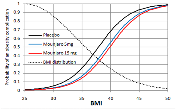
Figure 2
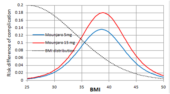
Figure 2 shows the expected risk reduction on Mounjaro 5 and 15mg weekly at each baseline BMI. The greatest point risk reduction 0.18 is at a BMI of 38. At a BMI of 30, the risk reduction is 0.03. At a BMI of 35, the risk reduction is about 0.12. The dotted black lines in Figures 1 and 2 indicate an estimated ‘Bayesian’ probability distribution (pending updating data) of BMI in the population. Moving the threshold for treatment from 30 to 35 would reduce the populations treated substantially. There will be stochastic variation about these points of course.
Curves such as those in Figures 1 and 2 would have to be developed for each complication of obesity. If a decision to take Mounjaro is shared using a formal decision analysis, the probability of each complication conditional on the individual patients BMI and its utility has to be considered as well as the demands of weekly injections possibly for life. In the USA, this would also involve the cost of medication and medical supervision. The decision analysis would have to compare the expected utilities of Mounjaro, lifestyle modification and no intervention at all.
Is this a fair representation of the difficult problem faced by primary care physicians in the UK when trying to interpret the result of the Mounjaro RCT?
- Jastreboff et al. Tirzepatide Once Weekly for the Treatment of Obesity. N Engl J Med 2022;387:205-216.
2 Likes
Regarding this topic, I have just posted the reply below to @Stephen on Deborah Mayo’s Error Statistics blog. I would be grateful for comments.
Thank you, Stephen, for making time to reply. I think that we agree on the points that you make. I will summarise the thinking in my paper (https://arxiv.org/pdf/2403.16906) to save you time for when you (or anyone else) can read more:
My understanding of the replication crisis is that
A. As you say, basing the frequency of replication on one second study of the same size gives a pessimistic result – the estimated frequency should be based on a second study of infinite samples size to simulate a ‘long view’ (see the first paragraph below).
B. My reasoning leads me to wonder that the current method of estimating required sample sizes overestimates power and underestimates the sample size required (by half), thus compounding the replication crisis (see the 2nd paragraph below).
C. An underestimate of sample size, and regarding a single identical study as a basis for replication, may explain the replication crisis (see the 3rd paragraph below) .
If a real first study result was based on 205 observations and its distribution happened to have a mean / delta of 1.96 and a SD of 10 then assuming a uniform prior, the Gaussian probability distribution of the possible true means conditional on this data has a mean also of 1.96 and a variance of 10/√205 = 0.698. If we consider all the possible likelihood distributions of the observed results of the second replicating study conditional on each possible true values, this represents the convolution of two Gaussian distributions. Therefore, the resultant probability distribution of the expected observed values in the second replicating study also getting P ≤ 0.05 has a variance of 0.698+0.698 = 1.397 and a SD of √1.397= 0.988. Based on these calculations, probability of getting P ≤ 0.05 again in the second replicating study is 0.5 as suggested by Goodman. However, if the sample size of the second study is infinitely large as suggested by you Stephen to simulate a ‘long view’, then the variance and SD of the second replicating study is zero and there is an overall variance is 0+0.698 and an SEM of 0.698 giving a probability of 0.8 of replication with P ≤ 0.05 again.
Conventional sample size calculations use a point estimate of the true mean / delta, (e.g. of 1.96) and an estimate of a SD (e.g. of 10) of the likelihood distribution of the imagined data in the ‘thought experiment’ on which the delta and SD were based. We can then estimate the sample size needed to get the necessary SEM to achieve a specified P value for the thought experiment data and the real study. However, instead of a likelihood distribution of the thought experiment data conditional on as single point estimate of a true mean of 1.96, we regard the above estimated distribution as a Gaussian probability distribution of the possible true means conditional on the thought experiment data. Then, the SEM of the data distribution in the real study after a convolution of two Gaussian distributions will be twice that of the above SEM (e.g. √0.698 x 2 = √1.397 = 0.988 as in the preceding paragraph giving a probability of 0.5 of getting P ≤ 0.05 in the real study of the same size as the 'thought experiment (the same as replication for a study of the same size in the preceding paragraph). Therefore, to expect P ≤ 0.05 in the real study with a probability of 0.8, we need a sample size of approximately twice 205 = 410. This sample size will then provide a correct probability of 0.8 of also getting P ≤ 0.05 in the real study based on two variances. If a replicating study is of theoretically of infinite sample size as suggested by you Stephen, the probability of replication will be 0.8 also. In this situation, there is no apparent replication crisis provided that the power calculation is based on two variances.
The real study must have the same sample size as that estimated for the ‘thought experiment’. This suggests that a conventional sample size estimate of 205 will be underpowered, only providing a probability of about 0.5 of getting P ≤ 0.05 in the real study. The probability of getting P ≤ 0.05 also in the real study’s replicating study conditional on the thought experiment and an underestimated sample size of 205 will depend on 3 variances and will provide a probability of replication of approximately 0.367, which is what was discovered in the Open Science Collaboration study. This suggests that the currently conventional estimates of sample size (e.g. giving a sample size of 205 as in the first paragraph) will cause real studies to be underpowered (e.g. at about 50% instead of the desired 80%) and the frequency replication of a single study of the same size will be alarmingly, but incorrectly, low (e.g. about 0.367). This underestimate of sample size, and regarding a single identical study as a basis for replication, may explain the replication crisis.
This avoids your excellent questions, but I feel that the use of null hypotheses is at the center of the replication crisis. A Bayesian sequential design like this one IMHO avoids much of the problem by demanding that 3 criteria be met:
- high probability of effect > 0
- moderately high probability of effect > trivial
- sufficient precision in estimating the treatment effect
Bayesian sequential designs also invite us to think about study continuation rather than study replication.
1 Like
Thank you Frank
The probability of getting a P ≤ 0.05 or P ≤ 0.025 based on the null hypothesis threshold of course can be replaced in my reasoning by a probability of >0.975 of the true result being less extreme than the null hypothesis or a probability of > 0.95 that the true result will be within the lower limit less extreme than the null hypothesis and the upper limit 2x1.96 SEMs less extreme that the null hypothesis (i.e. corresponding to 95% confidence interval). I can also replace the null hypothesis by some other less trivial threshold that takes account of clinical significance in the form of a greater required effect in the real study that is about to take place.
When the real result of a study has been observed, we can estimate the probability of replication with the same sample size for our chosen threshold without simply doubling it. The alternative calculation would be based on the convolution of the ‘Bayesian like’ first thought experiment distribution used in planning, with the second observed distribution. The sample sizes would be the same in both distributions but the resulting mean of the final distribution should be different to that obtained by doubling the variance. It would also be possible to apply Bayes rule to combine the thought experiment distribution with the real result’s distribution to double the number of observations in the ‘real’ result and halve the variance of the second distribution to be combined with the initial thought experiment in the convolution calculation.
Perhaps all the above could be used as part of a Bayesian sequential analysis too. I have not read the Bayesian Clinical Trial Design paper in detail but does it implicitly apply double the sample size obtained from a conventional Frequentist calculation in the way that I have done?
The more I read through this thread, the less clear it is to me on what is being conditioned upon, (ie. treated as fixed), and what is being allowed to vary.
If by “replicating” a study, you mean a future estimate is “close” (with “close” being undefined for now) to a previously reported estimate, that would require some way of down weighting the observed result, because treating a sample estimate as the true parameter almost certainly overestimates the confidence (in a frequentist sense) we should have in our estimate of a treatment effect. This is easy to do in a Bayesian framework, but less clear (to me at least) how to do so in a frequentist sense without a lot of data.
See this thread for a closely related discussion:
If by “replicate” you mean “obtain p < 0.05 and the estimates have the same sign” you face a similar problem. For the sake of argument, we will ignore that. Conditioning on the observed estimate (ie. treating the estimate as the true parameter value), we should expect at least half of our future studies to fail to achieve the same p-value (although they will likely have the same sign relative to N(0,1)), since the one-tailed p-value of the MLE is 0.5 (ie. the 50th percentile) in the N(\theta,1) scenario, where the non-centrality (or shift) parameter \theta \ne 0.
The fundamental problem is granting the p-value excess importance. It is the estimate that is a sufficient statistic, not the p-value, which is directly related to sample size and can change from sample to sample even if the sample size is kept constant under repeated sampling. It seems strange to define “replication” in terms of the realization of a uniformly distributed random quantity.
2 Likes
As you imply, the probability of replication depends on the chosen definition of the latter and the chosen evidence on which it is conditioned. The Open Science Collaboration study defined replication as discovering P≤0.05 again in a second study after discovering P≤0.05 in the first study. They recorded the frequency of this happening and found it to be 35/97 = 36.1%. They did not look at how often studies with P>0.05 had P≤0.05 in the second study (the total number may have been similar at 35). However, they stated that the 97 studies with P≤0.05 had been ‘well powered’ suggesting that there should have been a probability of at least 0.8 of that first study showing P≤0.05 and a probability of at least 0.5 of this also happening in the second study conditional on the pre-study planning estimates. However, instead of such a theoretical 50% frequency, the Open Science Collaboration study found it to be only 16.1%.
During their sample size calculation based on desired power, I assume that the investigators had chosen 80% power and a point estimate of the true mean of differences (or delta) and standard deviation. Based on the planning estimate’s sample size, they would then expect the above result. However, my point is that during their power calculation, they should take the variance of the planning estimate and that of the first study into account, which means that they need twice the estimated sample size to get a true 80% power. I am suggesting that this doubling of variance would give them a ‘true’ probability of 0.8 of getting P≤0.05 in the first study and 0.5 of getting P≤0.05 in the second, replicating study. However, by only basing their power calculation on a single variance and the resulting small sample size, they would only have a true 50% power for getting P≤0.05 in the first study and about 16.7% in the second study of the same sample size, which is what they got.
Another important point by @Stephen in the past is that a single replication study or many studies of the same size tells you little. It would be more sensible to look at a large number of such identical replicating studies and pooling their results or doing one study of huge sample size. If we imagine doing a second study of infinite sample size, then its variance would be zero, so that the probability of the second study replicating the first study with P≤0.05 again conditional on the imaginary planning estimate would be 0.8, the same as for the first study. However, if we are given a study result out of the blue and used this alone (without taking into account any planning estimate) the probability of replicating with a repeat study of infinitely large sample size would be calculated using one variance based on the sample size, observed mean and observed standard deviation of the out of the blue study. If we wish to calculate the probability of it being replicated by a study of the SAME size with P≤0.05, we would double the variance. If the latter probability turned out to be 0.8, then the probability of replication with P≤0.05 based on a study of infinite sample size based on a single variance would be about 0.977.
If we replace the probability of getting a P value of P≤0.05 with a 95% confidence interval or the probability of the true mean being greater than or less than zero or some other threshold, then the probability of replicating the latter will be the same as the probability of getting a P value of P≤0.05 as they are all directly related.
1 Like
You refer to:
I’m very skeptical of anything psychologists publish, given that they naively use parametric methods on ordinal data. I never felt comfortable using assessments designed like this, and I finally convinced myself it produces no information, which I argued in this thread. You can’t rely on their statistics without a laborous examination of of the included studies.
I have much more confidence in these publications, which are closely related to the questions you bring up in this thread:
van Zwet, E., Gelman, A., Greenland, S., Imbens, G., Schwab, S., & Goodman, S. N. (2023). A new look at P values for randomized clinical trials. Nejm evidence, 3(1), EVIDoa2300003.
van Zwet, E. W., & Goodman, S. N. (2022). How large should the next study be? Predictive power and sample size requirements for replication studies. Statistics in Medicine, 41(16), 3090-3101. (link)
Goodman, S. N. (1992). A comment on replication, p‐values and evidence. Statistics in medicine, 11(7), 875-879. (link)
2 Likes
My reason for using the Open Science Collaboration study was to give a real example in answer to your concerns about various definitions of replication and the evidence on which they are based. Its findings are consistent with those of other publications on replication. My suggestion is that the power and probability of replication should not be based on a single variance (that is current practice) except in special cases. This issue could contribute significantly to low probabilities of replication (depending on how we define the latter). I accept of course that there are many other causes for apparent and poor replication as observed in empirical studies as you point out and as described in the paper papers to which you refer.
1 Like
I think @f2harrell had the right idea in a prior post where he wrote:
People need to give up on the idea that p values under the reference null are important. Designing studies to achieve a particular p-value are not economical when you look at the required sample sizes.
The reference distribution N(0,1) is just that – a starting point from which we can define any deviation from as information (in a mathematical sense). After there are a number of estimates available, deviation of an estimate from the reference distribution N(0,1) is no longer relevant. We can compare 2 observed Z scores directly via the modification of the Stouffer/Liptak nonparametric combination method. Assuming 2 studies are a sampled from the same normal distribution, a quick test of heterogeneity for 2 statistics is:
\frac{Z_2 - Z_1}{\sqrt{2}}
This was discussed in:
Wolf, F. M. (1986). Meta-analysis: Quantitative methods for research synthesis (Vol. 59). Sage, p. 43-44.
It wasn’t clear from the text, but if I were given 2 Z scores, I’d assign Z_2 = max and Z_1 = min of the score pairs, so deviations in sign are treated correctly. Two observations in opposite tails of the distibution should be very unlikely.
2 Likes
Well said. After a fun week discussing this work with @EvZ, very much agree that these references are very relevant here.
1 Like
In their introduction, Van Zwet (@EvZ) and Goodman (https://onlinelibrary.wiley.com/doi/full/10.1002/sim.9406) point to the Open Science Collaboration paper (their first reference) as “the most widely known empirical examples. This realization has given rise to the so-called replication crisis”. Unlike you @R_cubed, they accepted this result at face value with no overt scepticism at least! I had predicted the Open Science Collaboration paper result of about 16% correctly by assuming that their power calculation had been based incorrectly on one variance rather than correctly with two or three or adding the component variances (see Equation 13 in my paper (see https://arxiv.org/pdf/2403.16906 ).
Van Zwet and Goodman also state in their Abstract that “an exact replication of a marginally significant result with P = 0.05 has less than 30% chance of again reaching significance. Moreover, the replication of a result with 0.005 still has only 50% chance of significance”. In Equation 1 of my own paper I estimated that the frequency of such replication based on an correct double variance and original P = 0.025 one sided would be about 28.3%. Furthermore, in Equation 6 of my paper, if an original P was 0.0025 one sided, then when correctly using a double variance in the calculation the real observed frequency of replication would be about 51%. Therefore, I predicted the findings in the Van Zwet and Goodman paper correctly by assuming that the power was estimated correctly with two variances and not in the currently conventional way by using only one variance. The latter overestimates power and underestimates the correct sample size needed, thus causing or at least contributing to the replication crisis.
The same problem will arise not only when power is calculated for simple P values but also for effect-size & power-focused calculations using Z scores etc. as suggested by you and also perhaps by @f2harrell. So my suggestion is that the current replication crisis may be due mainly to errors in calculating the required sample size by using only one variance when planning a study and also when estimating its probability of replication.
I would be happy to debate the validity of these results from psychological studies with them. When 2 mathematical psychologists (Joel Michell and Paul Barret) characterize psychometrics as a “pathological science”, and the entire “replication crisis” is centered in psychology, I think it is reasonable to severely discount anything coming out of that area of study.
They aren’t the only ones who argue that psychological data is at best ordinal, and should be statistically examined using ordinal methods. Psychologist Norman Cliff published 2 books on ordinal methods that share many similarities with the recommendations of @f2harrell, even though he didn’t go into as much detail on the proportional odds model.
Suffice it to say, the Cochrane Database of medical RCTs is more relevant to your question.
Related Thread:
Although various statistical methods are available for the analysis of PROs in RCT settings, there is no consensus on what statistical methods are the most appropriate for use.
Instead of deriving the right path from first principles, they go through a fruitless exercise of empirically fitting various models, much like is done in psychometrics. But they are correct in that most researchers argue about how to properly analyze the data, with those favoring treating ordinal data as interval having positions of authority. That makes the reported statistics useless, and also makes any meta-analysis also worthless.
2 Likes
Having been on the front lines of data analysis in biomedical research for decades, and being a casual observer of data analysis in quantitative psychology, I’m not so sure that psychology is worse. I am constantly sickened by what I see in biomedicine.
This makes me think that replication probability should be de-emphasized and instead efforts should be focused on designing perfect studies then seeing what you can do to make a feasible study have as many of the qualities of the perfect study as possible. A small part of that might include calculation of the margin of error in estimating a key estimand, when the sample size is ‘safely large’ and comparing that to the margin of error achieved when doing the usual sample size samba.
3 Likes
I’m having some difficulty with section 6.1 of your paper on ArXiv. I’ll introduce some notation. Let beta denote the (unobserved) true effect effect of the treatment and let b be a normally distributed estimator with mean beta (i.e. b is unbiased) and (known) standard error s. Define the z-statistic z=b/s and the signal-to-noise ratio SNR=beta/s.
The z-statistic has the normal distribution with mean SNR and standard deviation 1. In other words, z is the sum of SNR and an independent standard normal error. If there is no effect (beta=0) then SNR=0, so z has the standard normal distribution. In that case the probability that z exceeds 1.96 is 0.025.
Now, let z_repl be the z-statistic of a replication experiment with the same signal-to-noise ratio as the original experiment. So, z_repl is the sum of the same SNR but another independent standard normal error.
If we assume that SNR has the (improper) uniform distribution, then the conditional distribution of SNR given z, is normal with mean z and standard deviation 1. If follows that the conditional distribution of z_repl given z, is normal with mean z and standard deviation sqrt(2).
In the example from section 6.1, you have b=1.96, s=1 and z=1.96. Given z=1.96, the SNR has the normal distribution with mean 1.96 and standard deviation 1, and z_repl has the normal distribution with mean 1.96 and standard deviation sqrt(2). Therefore, the conditional probability that z_repl exceeds 1.96 is 0.5. This is the probability of “successful replication” in your example. In other words, if SNR has the uniform distribution then
P(z_repl > 1.96 | z=1.96) = 0.5.
In section 6.1, you compute the conditional probability that z_repl > 2.77. That is,
P(z_repl > 2.77 | z=1.96) = 0.283.
I don’t understand why you compute this particular probability. I do not think it’s “the probability of getting a P-value of 0.025 or less when the study is repeated with the same number of observations” as you say.
Steve Goodman computed the probability of “successful replication” assuming the uniform distribution for the SNR in his 1992 paper “A comment on replication, P-values and evidence”. He called it the “predictive power”. In the paper of Steve and me from 2022, we replaced the uniform distribution by a distribution which we estimated across the Cochrane Databse of Systematic Reviews.
4 Likes
If I made 100 observations and discovered a mean of 1.96 and standard deviation of 10, by assuming uniform priors the probability distribution of true means is represented by the double blue line that has a mean of 1.96 and a SEM of 10/√100 = 1.
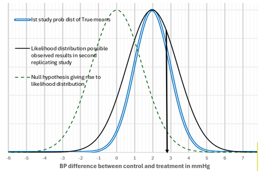
If for each of the possible true means on this distribution, I perform the same study with a SEM of 1, then the distribution of possible observation values in the second study will be represented by the black line distribution with an SEM of √(1+1) = 1.414 with a mean of 1.96 and an SEM of 1.414. This is a convolution of two identical Gaussian distributions, each represented by the double blue line. If we specify a null hypothesis of zero for this new distribution, then it is represented by the green dotted line. The 1.96 SEMs away from zero with an SEM of 1.414 mmHg is 1.96x1.414 = 2.77mmHg difference from zero (see the black down arrow). The area to the right of the black arrow and the black distribution line is 28.3% of the total area bound by the black distribution line. In other words of all the possible observations in the second study, 28.3% will give a P value of less than or equal to 0.025. Therefore, the probability of the second replicating study giving P≤0.025 one sided is 0.283.
I guess we’re not talking about the same thing. So let’s first see if we agree on the math. I claim that if the SNR has the (improper) uniform distribution then
P( z_repl > 1.96 | z=1.96) = 0.5
and
P( z_repl > 2.77 | z=1.96) = 0.283
Do you agree?
Now, I call the former the conditional probability of “successful replication” given z=1.96. You the latter?
I call P( z_repl > 2.77 | z=1.96) = 0.283 the probability of replication with P≤0.025 one sided or P≤0.05 two sided when the null hypothesis is zero and the variance is 1+1 and the SEM is 1.414.
Am I correct that you are also implying the following (or have I misunderstood)?:
- P( z_repl > 1.96 | z=1.96) = 0.5 when SEM = 1 and 1.414 or any other SEM. Does this also imply that P(P≤0.05 two sided or P≤0.025 one sided | z= 1.96) = 0.5?
Also - P( z_repl > 0 | z=1.96) = 0.975 when SEM = 1
- P( z_repl > 0 | z=1.96) = 0.917 when SEM = 1.414 (when variance is 1+1)
- P( z_repl > 2.77 | z=1.96) = 0.283 when SEM = 1.414 (when variance is 1+1)
- P( z_repl > 2.77 | z=1.96) = 0.208 when SEM = 1
Kileen (2005) referred to Equation 3 as the ‘P-rep’. However, for better or worse ‘replication’ has been regarded widely as not only getting a difference in the same direction and also P≤0.05 two sided or P≤0.025 one sided. Equation 4 represents the latter probability according to the reasoning set out in my previous post. If you describe Equation 1 as the conditional probability of “successful replication”, what would you call the other equations, and in particular, Equation 4?
1 Like