Some thoughts on uniform prior probabilities when estimating P values and confidence intervals

I agree of course. If from the above reasoning, I get P=0.05 in a study with a difference of 2.0mmHg and SD = 10 but it was originally underpowered with only 100 observations, then the probability of replication is only 0.283:
NORMSDIST(1.96/(((10/100^0.5)^2)*2)^0.5+NORMSINV(0.05/2)) = 0.283 (Equation 3)
In this case P=0.05 was a fluke and unlikely to be replicated. The calculation is only based on 2 variances because any power calculation performed in the planning stage that estimated the result of the first study has been overtaken by the actual result of the first study. The probability of replication in the second study is therefore based only on the observed outcome of the first study and their (two) respective variances.

However, if I got P=0.05 from a study that had been well powered with 409 observations then the probability of replication would be 0.8:
NORMSDIST(1.96/(((10/409^0.5)^2)*2)^0.5+NORMSINV(0.05/2)) = 0.800 (Equation 4)
This is more solid result less due to chance and more probably replicated. Note that the P = 0.05, the difference from zero and SD are the same on both occasions so without estimating the probability of replication based on the number of observations on which it was based, the P value provides limited evidence. Statisticians are already aware intuitively of this nuance but perhaps the above reasoning will help get the nuance across to non-statisticians.

A Bayesian approach may give a different impression.

The estimated prior distribution of the expected result of the study makes a significant impression on these approaches too of course.

If I had done the power calculation to estimate the number of required observations using a subjective distribution with an estimated BP difference from zero of 1.96mmHg and a SD of 10, then the number of observations needed to get P≀0.05 in the replicating study, would have been 613:
(10/(((1.96/(NORMSINV(0.8)-NORMSINV(0.05/2)))^2)/3)^0.5)^2 = 612.9 (Equation 5)

If the resulting first study came up with a BP difference of 1.96mmHg, then by using this to estimate the probability of replication based two variances with 613 observations, we get a probability of replication of 0.913:
NORMSDIST(1.96/(((10/613^0.5)^2)*2)^0.5+NORMSINV(0.025)) = 0.929. (Equation 6)

If the result of the first study happened show a BP difference of 1.6mmHg based on 613 observations, then the probability of replication based on 2 variances is 0.801, indicating that a P value above 0.05 could be a useful result:
NORMSDIST(1.6/(((10/613^0.5)^2)*2)^0.5+NORMSINV(0.025)) = 0.801 (Equation 7)

Does this bear a resemblance to the usual Bayesian approach?

If I had done the conventional power calculation to estimate the number of required observations based on an estimated BP difference from zero of 2.197mmHg and a SD of 10, then the number of observations required for a power of 80% to get P≀0.05 for the first study would be 163:
(10/(((2.197/(NORMSINV(0.8)-NORMSINV(0.05/2)))^2)/1)^0.5)^2 = 162.6 (Equation 8)

If we assume the Bayesian prior distribution had the same or similar SD of 10 and difference from zero of 2.197 and P=0.028, then by combining the Bayesian prior with the actual result, we end up with a posterior distribution with similar variance and difference but twice the number of observations of 163+163 = 326. If we now use this Bayesian ‘posterior’ distribution result from the first study to estimate the probability of replication with a P≀0.05 in the second study using the 2 variance formula, we get:
NORMSDIST(2.197/(((10/326^0.5)^2)*2)^0.5+NORMSINV(0.025)) = 0.801 (Equation 9)

On this occasion, the ‘Bayesian’ reasoning gives the same result as Equation 2 in Post 19. A different prior Bayesian distribution would give a different result of course. Does this make sense?

If I understand, there are 2 remaining issues:

  • you are still getting evidence for non-zero effects instead of the likely more relevant evidence for non-trivial effects when computing p-values
  • an SD of 10 in the raw data is not relevant for the SD of the prior for an effect

I take your point. I tried to combine the estimated distribution as if it were a Bayesian prior distribution based on knowledge of the proposed study, with the actual result of the first study to get a posterior estimation. I agree that the reasoning doesn’t work in this setting. I will therefore use the term ‘Bayesian-like’ because I don’t intend to use the estimated distribution in a Bayesian manner by combining it with a likelihood distribution to get a posterior distribution. It is the following five approaches (A) to (E) that I am proposing as being legitimate:

(A) To estimate the probability of replication ‘x’ to get P≀y (1 sided) in a second study when the first study’s observations are known already: (i.e. (1) the number ‘n’ of observations made, (2) the observed difference ‘d’ of the mean from zero and (3) the observed standard deviation ‘s’). This approach is based on doubling (*2 in the formula below) the variance being calculated from the above 3 observations.
x = NORMSDIST(d/(((s/n^0.5)^2)*2)^0.5+NORMSINV(y)) Equation 10

(B) To estimate the number of observations ‘n’ needed for a power of ‘x’ to get P≀y (1 sided) in the first study from a ‘Bayesian-like’ prior distribution based on prior knowledge of the planned study that allows an estimate to be made of the difference of the mean from zero ‘d’ and an estimated standard deviation ‘s’. This calculation involves doubling the variance of the Bayesian-like prior distribution (applied by ‘/2’ in the formula below).
n = (s/(((d/(NORMSINV(x)-NORMSINV(y)))^2)/2)^0.5)^2 Equation 11

(C) To estimate the number of observations needed for a power of x to get P≀y 1-sided in the second study from a ‘Bayesian-like’ prior distribution based on an estimated difference of mean from zero ‘d’ and an estimated standard deviation ‘s’. This calculation involves tripling the variance of the Bayesian-like distribution (applied by ‘/3’ in the formula below).
n = (s/(((d/(NORMSINV(x)-NORMSINV(y/2)))^2)/3)^0.5)^2 Equation 12

(D) A ‘what if’ calculation based on the above Bayesian-like distribution by calculating the probability of replication ‘x’ of the first study based on doubling the variance of the Bayesian-like distribution (applied by ‘/2’ in the formula below) and by inserting various observation numbers ‘n’, various values of the difference of the mean from zero (d), the standard deviation (s) and the desired a 1-sided P value ‘y’, into the expression. This can be used for sensitivity analyses of the parameters of the Bayesian distribution.
x = NORMSDIST(d/(((s/n^0.5)^2)*2)^0.5+NORMSINV(y)) Equation 13

(E) A ‘what if’ calculation based on the above Bayesian-like distribution by calculating the probability of replication ‘x’ of the first study based on tripling the variance of the Bayesian-like distribution (applied by ‘/3’ in the formula below) and by inserting various observation numbers ‘n’, various values of the difference of the mean from zero (d), the standard deviation (s) and the desired a 1-sided P value ‘y’, into the expression. This can be used for sensitivity analyses of the parameters of the Bayesian distribution.
x = NORMSDIST(d/(((s/n^0.5)^2)*3)^0.5+NORMSINV(y)) Equation 14

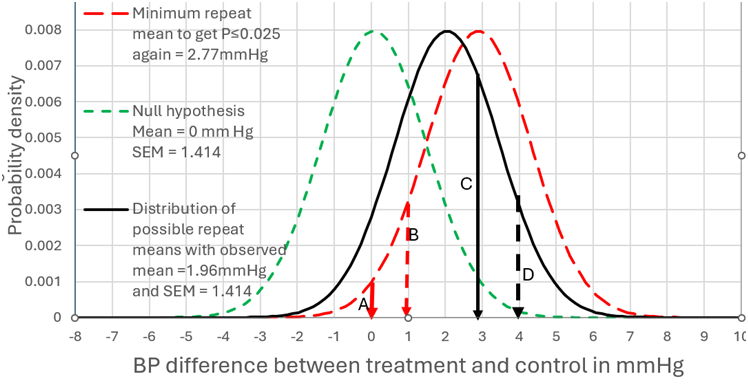
I will address your interesting point about non trivial differences. The best diagram I have is with the example of a mean difference of 1.96mmHg BP difference and a SD of 10. Figure 1 can therefore represent scenario (A) when the number of observations was 100. In this case there was a probability of replication of 0.283 for a one sided P value:
=NORMSDIST(1.96/(((10/100^0.5)^2)*2)^0.5+NORMSINV(0.025)) = 0.283 Equation 15
This corresponds to the area to the right of arrow C of the distribution under the black unbroken line) where P≀0.025 in the replicating study (i.e. all BP differences ≄2.77mmHg).

By assuming that the prior probability conditional on the set of all numbers is uniform (i.e. prior to knowing the nature of the study), then when P=0.025, the probability of the true value being a BP difference of ≄0mm Hg is 0.975 (see the area to the right of arrow A in Figure 1 under the green dotted distribution). For a non trivial difference of 1mmHg BP we look at the area to the right of arrow B, where the probability of the true value being a BP difference of ≄1mm Hg is 0.831 and P=0.169 (1-0.831). The probability of getting the same result again is also 0.283.

If we move the arrow C to D (from a BP difference of 2.77mmHg to 3.77mmHg) then this BP difference of ≄3.77mmHg accounts for 10% of the results. They correspond to P≀0.003824 for the green dotted distribution at the broken black arrow D. The probability of the true value being a BP difference of ≄0mm Hg conditional on a result mean of 3.77mmHg is 0.996176 (1-0.003824). This is represented in Figure 1 by moving the red dotted distribution from a mean of 2.77mmHg (the big black arrow) so that the mean is 3.77mmHg (the small broken arrow D). However, the probability of the true value being a BP difference of ≄1mm Hg conditional on an observed mean of 3.77mmHg is 0.975. There is a probability of 0.100 that this will also be the case if the study is repeated (corresponding to the area under the black unbroken distribution to the right of arrow D).
NORMSDIST(1.96/(((10/100^0.5)^2)*2)^0.5+NORMSINV(0.003824))=0.100 Equation 16

Figure 1:

image

In conclusion, these arguments depend on a number of principles:

  1. The prior probability of each possible result of a study is uniform conditional on the universal set of rational numbers (and before the nature of a proposed study, its design etc is known). This means for example that the probability of a result being greater than zero after continuing a study until there is an infinite number of observations, equals 1-P if the null hypothesis is zero.
  2. The Bayesian-like prior probability distribution of all possible true results is a personal estimation conditional on knowledge of a proposed study and estimation of the distribution’s various parameters.
  3. During calculations of a probability of achieving a specified P value, of replication of a first study by a second study, estimation of statistical power or the number of observations required, this Bayesian-like distribution is not combined with real data to arrive at a posterior distribution, but its estimated variance is doubled or tripled.
1 Like

Looks good. Just consider using a small prior SD on the true mean difference.

A pure Bayesian look at the problem might be emphasizing Pr(effect > c | study 1 data, prior) and Pr(effect > c | study 1 and study 2 data, prior).

A side remark: Frequentist multiplicity comes largely from asking too little from the data, i.e., trying to get evidence against an exactly zero effect. When you calculate Pr(union of events that are all easy to achieve) e.g. Pr(treatment effect > 0 on one thing or effect > 0 on other thing) this compound probability can easily be high. When you replace 0 with c (c > 0) not so much.

1 Like

My main point is that the replication crisis might be due to the current frequentist method of estimating sample sizes during power calculations. This is because they appear to underestimate the number of observations required for the first study and do not estimate the numbers required for the second study at all. According to my reasoning if in a crossover study the observed BP difference minus zero was 1.96mmHg with a standard deviation of 10mmHg, then in order to get a one-sided P value of 0.025 or less in the first study, we would require 409 observations by applying double the variance of the prior estimate (‘/2’ below):
(10/(((1.96/(NORMSINV(0.8)-NORMSINV(0.025)))^2)/2)^0.5)^2 = 408.6 Equation 17

However, the conventional frequentist estimate is only based on the (single) variance of the prior distribution (‘/1’ below):
(10/(((1.96/(NORMSINV(0.8)-NORMSINV(0.025)))^2)/1)^0.5)^2 – 204.3 (Equation 18).

Do you think that the results of Pr(effect > c | study 1 data, prior) and Pr(effect > c | study 1 and study 2 data, prior) affect the estimations of the number of observations required according to Equation 17 or Equation 5 (or in general terms Equations 11 and 12)?

1 Like

Yes I think that would meaningfully affect the calculations. There is also a philosophical question: Should study 2 be informed by any results from study 1? Should a Bayesian approach just treat Study 2 as a continuation of Study 1 so that the posterior can be sharpened (I think so).

1 Like

Thank you. I suppose the only way to solve the problem is to make different assumptions, calculate the estimated the probability of replication, record how often the replication occurred and then see which calculation resulted in a calibration curve of estimated numbers of observations that was nearest to a line of identity after study similar to that conducted by the Open Science Collaboration!

When Frequentists estimate the number of observations to achieve a specified power of getting P up to a specified value, they too are making a prior subjective estimate based on effect size. However, they do not bring that prior estimate into their calculation by adding its variance to the identical expected variance of the first study. They only base their calculation on the expected variance of that first study based on their prior estimate.

What I propose is basing the estimate of the required number of observations on a ‘double variance’ in a calculation that incorporates the estimated prior distribution. I do not use the term ‘Bayesian’ because the calculation does not use Bayes rule. Instead of a Bayesian multiplication, the calculation involves addition because the second identical probability (not likelihood) distribution is summated on each possible result of the first estimated prior distribution to create a new 3rd distribution with an SEM that is double the original SEM. In order to estimate the probability of replication in a second study the process is continued because the original distribution is summated on each possible result of the 3rd distribution to create a 4th distribution with an SEM that is triple the original SEM. In terms of Bayesian philosophy, I have already incorporated the prior distribution and doing it again may exaggerate the probability of replication.

The Frequentist estimation of the numbers needed to get to get P≀0.25 with a difference of 1.96, a SD of 10 is 204.5. Incorporating the prior distribution gives 2 x 204.5= 409. However in order to get P≀0.25 in the second study, we need 409+204 = 613. If we use the latter during study, then the probability of getting P≀0.25 in the first study is 0.929
= NORMSDIST(1.96/(((10/613^0.5)^2)*2)^0.5+NORMSINV(0.025))= 0.929 (Equation 19). However, the latter takes into account a range of possible P values. If the P value happened to be 0.025 on the basis of 613 observations in the first study, the probability of getting 0.025 again in the second study conditional on this P value in the first study would be 0.929 again, the calculation being identical to Equation 19. Interestingly, if the first study’s P value happened to be 0.054 one-sided, the probability of replication in the second study based on 613 observations in the first study would still be 0.803:
=NORMSDIST(1.6)/(((10/613^0.5)^2)*2)^0.5+NORMSINV(0.025)) = 0.803 (Equation 20)

Because the prior distribution has already been taken into account, I’m not sure that a PLAN to incorporate the prior distribution into a Bayesian calculation could change the numbers required in the study. However, if the effect size and SEM in a completed study were very different to that in the original prior estimate, perhaps Pr(effect > c | study 1 data, prior) and Pr(effect > c | study 1 and study 2 data, prior) should be estimated. Unless there were a very big difference between the effect sizes and SEMs, the impact of the prior distribution might be muted as the number of observations on which the real outcome was based might be 2 or 3 times those in the prior distribution.

1 Like

There is a related literature on Bayesian sample size estimation with a key word of assurance. They do frequentlist-like calculations but with a continuous distribution for effect size instead of using the single MCID.

1 Like

Thank you again. I Googled 'Bayesian’ and ‘assurance’ and discovered this paper by Brus et al: Bayesian approach for sample size determination, illustrated with Soil Health Card data of Andhra Pradesh (India) (sciencedirectassets.com). Table 2 of this paper compares the results of applying the Frequentist approach and various Bayesian approaches to estimating sample size. The latter were 5% to 30% higher than the Frequentist estimates. I have not examined the details of the Bayesian calculations but superficially, they do not give similar results to the methods suggested by me and they do not address the issue of replication with a second study. This suggests that the Bayesian and the approach suggested by me for estimating sample size are based on different underlying assumptions.

Yes but it may be possible to blend the two, if it helps. I did one calculation here where replacing a point MCID of 0.65 with a uniform interval 0.55 yo 0.75 resulted in about 0.1 lower “Bayesian power”.

Does the Figure 1 below using my example of BP differences illustrate the same point (if I understand it correctly)?

Figure 1
image

FWIW, this 2022 paper published in Statistical Science by Micheloud and Held are directly relevant to this thread. Fortunately it is open access.

2 Likes

I think these are single-point-MCID conditional probabilities, no?

Sorry. I should have explained what I did more clearly.

I listed in Excel a range of MCIDs from 0.96 at 0.01 intervals up 2.96 and calculated the sample size required to get P≀0.05 two sided with a power of 80% at each MCID (the blue line in the Figure) using my usual expression:
=(10/(((MCID/(NORMSINV(0.8)-NORMSINV(0.05/2)))^2)/1)^0.5)^2

I then calculated the various powers obtained with the frequentist sample size of 204.3 (based on an assumed MCID of 1.96) for each listed MCID instead, using the expression:
=(NORMSDIST(MCID/(((10/204.3^0.5)^2)*1)^0.5+NORMSINV(0.025)))*100

These calculations were not weighted according to a prior probability distribution of each MCID (their distribution can therefore be regarded as ‘uniform’). However if a prior distribution had been specified, its expected or modal value would have been at 1.96mmHg BP difference. I suppose the prior probabilities of the possible MCIDs would be along the lines of Figure 2 (the dotted points were not in the above calculations, only those between 0.96 and 2.96):

Figure 2
image

This fixed \alpha and then choose \beta is not consistent with a Bayesian perspective, which minimizes a linear combination of \alpha and \beta.

1 Like

I’m not sure that I am operating within a Bayesian framework because I don’t use Bayes rule in my calculations. Instead of combining distributions by finding their products, I summate them by adding their variances.

What is wanted is not the MCID that achieves a certain power but rather the average (over MCID distribution, uniform or not) power.