I had already defined the symbols in the first version, this version was intended as a form of addendum to the former.
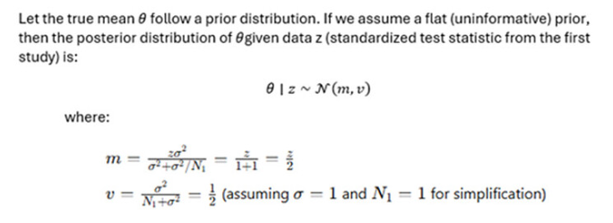
But theta does NOT have a uniform distribution. The uniform distribution has been updated by the information in the completed study to give a conditional (posterior) mean of z/2. It is this that gives a result of 0.292 that appears to give a realistic estimation of replication frequency (as opposed to 0.511 when the conditional variance is 1).
Let the true mean theta follow a prior distribution. If we assume a flat (uninformative) prior …
So you’re assuming that the prior of theta (i.e. before the first study) is the uniform distribution. Correct?
Now, if the prior of theta is the uniform distribution and z|theta ~ N(theta,1), then the posterior distribution of theta (i.e. after the first study) is normal with mean z (not z/2) and standard deviation1 (not 1/2).
Can you explain where you think that it was argued or implied by me that the conditional (posterior) mean of theta is z/2 and that the conditional variance of theta was 1/2?.
Thank you. I have been trying to guess what sort justification in mathematical notation that you expect on this topic and included provisionally at one point a closed-form formula that I omitted to delete, that specified an m=z/2 and v=1/2. This was of course irrelevant to the final expression, not part of it and should have been deleted to avoid confusion. My ‘double variance’ approach also aims to avoid exaggerating the strength of evidence so any other closed-form formula would be unnecessary.
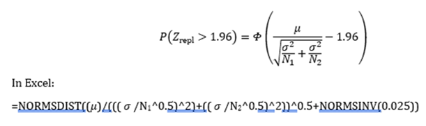
The assumptions that you want me to clarify seem best done verbally. Many are of course obvious such as the meaning of mean, standard deviation, variance etc. and their symbols. The main assumption that I make is that when trying to predict the results of one study from another, the variance of both need to be taken into account in the calculation by adding them to model a process of convolution. Also in a perfect model of a random selection, before anything is known about the process, the prior probabilities of theta and mu conditional on the universal set of all numbers can be assumed to be uniform. This is the resulting expression;
This expression simply represents a hypothesis which postulates the frequency of replication of future identical studies with P≤0.05 two-sided or Z>1.96, if the repeat study has the same mean and SD as the completed study and a specified number of samples. N1 = N2 being a special case. This postulate appears to be consistent with the results of the 2022 paper by you and Goodman. It is also appears consistent with the results of the Open Science Collaboration study.
I think that the statistical and scientific community should consider taking a look at this as a possible explanation of the replication crisis and how to fix it. If you need detailed clarification about anything, please ask.
I have been trying to guess what sort justification in mathematical notation that you expect on this topic
No need to guess – I can tell you (again). You use the terms “prior”, “likelihood” and “posterior” but those are only meaningful in the context of a complete and coherent probability model. For all your clever-sounding talk about postulates, random selection, the process of convolution, the universal set of all numbers or whatever else, you are evidently unable to provide such a model. In fact, I have serious doubts that a coherent model exists that would lead to your replication formula. The uniform prior will certainly not work.
Datamethods is a platform where people can share ideas and learn from each other. I am a professional statistician with a PhD in mathematics. I’ve been trying to explain what’s wrong with your preprint, but it’s become obvious that you don’t want to learn anything from me. You’re only interested in defending your preprint no matter what. So, I’m wasting my time. If I wanted to get into pointless debates, I’d go to 4chan.
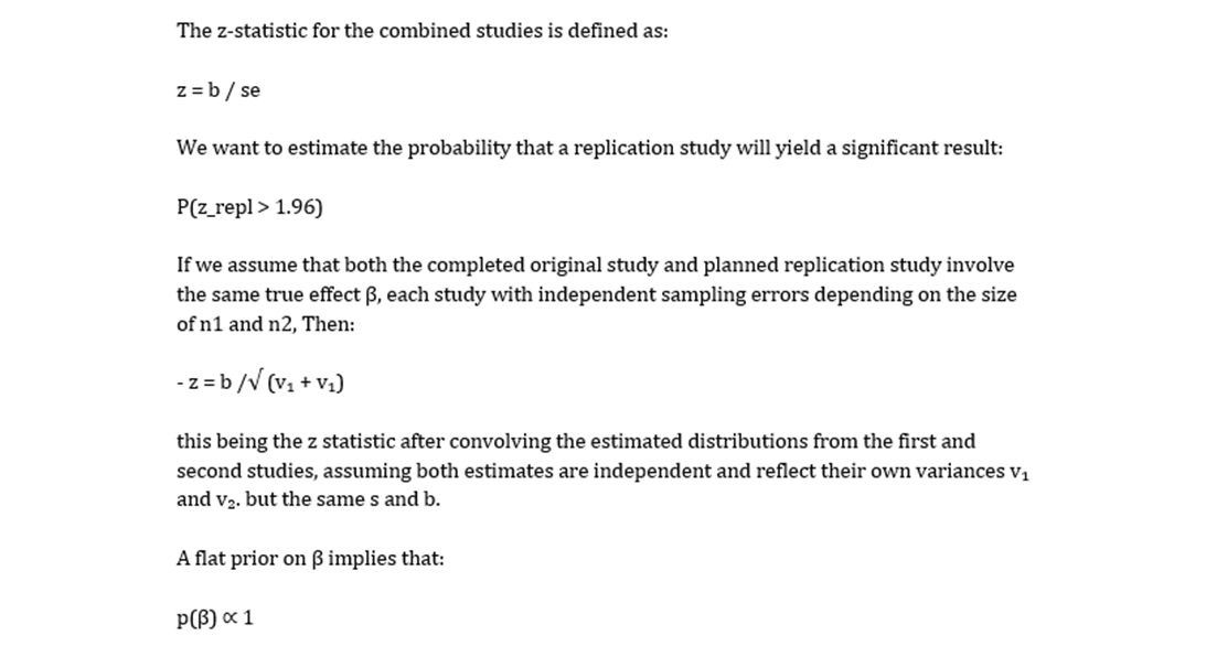
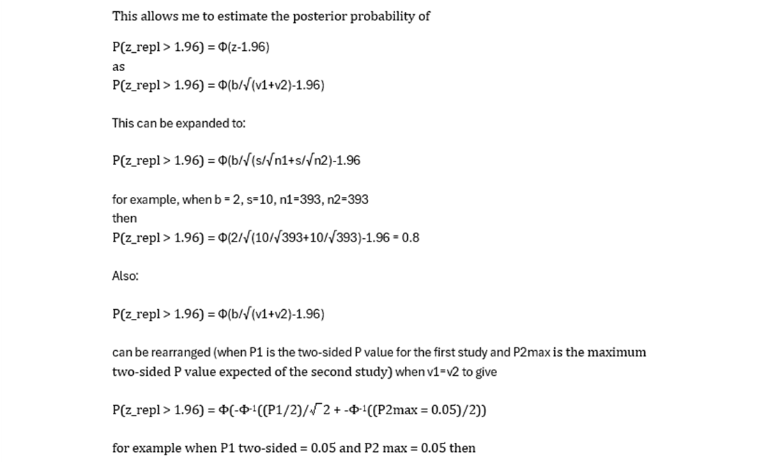
Thank you for that. The problem is that I express my concepts in Excel notation that allow me to explore their consequences numerically and graphically immediately in a dynamic way both theoretically and practically with real data. It means that this expression:
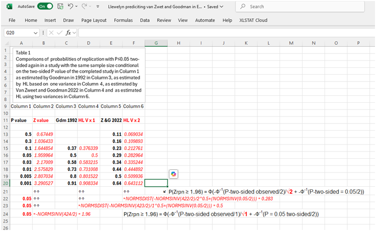
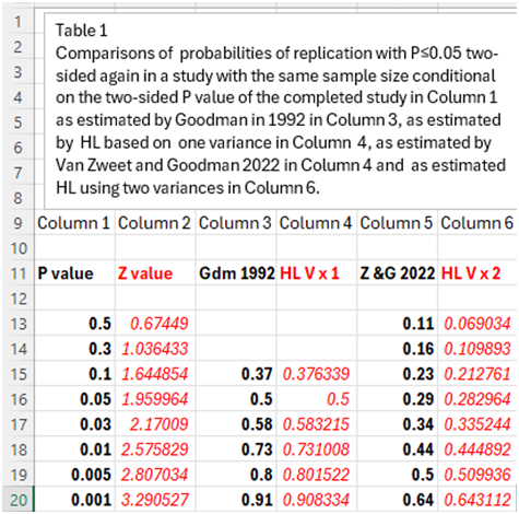
As shown in Table 1 below that displays an image of a Excel spreadsheet, the above expressions allow us to calculate in Excel the probabilities of replication directly (see column 6) from variously observed P values (see column 1). They match those computed by you and Goodman 2022 in column 5. Goodman in 1992 calculated probabilities of replication as in column 3. These correspond to my results if I replace two variances by one variance ( see the red characters) to get the results in column 4. Columns 3 and 4 overestimate the real results in column 5 discovered by you and Goodman in 2022 and by my expression based on 2 variances that predict them in column 6.
The problem is that you claim that this formula represents the posterior probability P(z_repl > 1.96 | z). To make such a claim, you need to specify a prior and a likelihood, and show that your posterior follows from them. You are clearly unable to do so. You say you’re using the uniform prior, but that is obviously not possible.
A further problem is that you seem to be under the impression that your formula is universal. In other words, that it represents the posterior probability of replication irrespective of the distribution of the SNR. I’ve tried to explain why that cannot be true, but – again – without making any impression on you.
I explain all this carefully in my paper. In random sampling, MU and THETA are on the same regular measurement scale with intervals of DELTA n, DELTA n+1, DELTA n+2 etc. The interval between DELTA n and DELTA n+1 and DELTA n+1 and DELTA n+2 etc. can be referred to as the constant ‘DELTA K’, which is often an unknown number and vanishingly small for continuous variables.
The prior probability p(MY I | USN) = DELTA-K is the probability of {MY i} conditional on the universal set of all numbers. Also as THETA is on the same scale, the prior probability p(THETA j| USN) = DELTA-K is the prior probability of {THETA j} conditional on the universal set of all numbers
A posterior probability is represented by p(THETA j | MU i) and a likelihood probability is represented by p(MU i | THETA j).
This means that by Bayes rule:
p(THETA j|USN) x p(MU i | THETA j) = p(MY i|USN) x p(THETA j | MU i)
and
p(THETA j|USN) / p(MY i|USN) = p(THETA j | MU i) / p(MU i | THETA j)
But as p(THETA j|USN) = p(MY i|USN)
then
p(THETA j | MU i) / p(MU i | THETA j) = 1
and
p(THETA j | MU i) = p(MU i | THETA j)
when there is random sampling so that {MU i } and {THETA j are on the same measurement scale (e.g. as continuous variables).
This also means that when modelling random sampling, the likelihood and posterior distributions are superimposed. For the purposed of convolution of two distributions both must be regarded as probability distributions and the resulting distribution based on two variances is also a probability distribution.
This is in contrast to a Bayesian calculation where a posterior probability distribution is based on a conditional prior probability distribution of possible values of THETA conditional on data MU1 (not conditional on the universal set of numbers) and a likelihood distribution is of data MU2 conditional on each possible value of THETA.
Because of a uniform prior probability distribution of THETA j and MU I conditional on the universal set, the order of discovery of MU1 and MU2 is immaterial. Therefore if data MU2 is discovered first, then the conditional prior probability is of all the possible values of THETA conditional on the data MU2. The likelihood distribution is of data MU1 is then conditional on each possible value of THETA.
You often talk about SNR that is rarely mentioned in medical statistics and RCT analysis (except when assessing imaging such as CT scans or MRI). Do you mean SNR as signal power over noise variance or SNR as signal over standard error? How do you think that their distributions would affect the calculation of P(Zrepln > 1.96? From what I have understood, the SNR distribution would not be relevant.
You still haven’t defined MU, THETA, DELTA, USN and MY.
The prior probability p(MY I | USN) = DELTA-K is the probability of {MY i} conditional on the universal set of all numbers.
This gibberish, even apart from the fact that you haven’t defined any of the symbols. The rest is gibberish too.
You often talk about SNR that is rarely mentioned in medical statistics
Contrary to you, I actually define my variables and their relations. As I’ve now written repeatedly without you taking the trouble to read:
Let beta denote the (unobserved) true effect effect of the treatment and let b be a normally distributed estimator with mean beta and (known) standard error s. Define the z-statistic z=b/s and the signal-to-noise ratio SNR=beta/s. The z-statistic then has the normal distribution with mean SNR and standard deviation 1. In other words, z is the sum of SNR and an independent standard normal error. Let z_repl be the sum of the same SNR, but another independent standard normal error.
In your set-up the standard error of the estimator (which I call “s”) is sigma/sqrt(N). I’ve used sigma to denote the standard deviation of the prior distribution of the SNR. I’ve also used mu to denote the mean of the prior distribution of the SNR.
The SNR is key because it links the two z-statistics. So, if you want to talk about P(z_repl > 1.96 | z) you must consider the distribution of the SNR. Now, please stop fighting me, and just go over my posts and try to understand what I’m explaining to you.
Even though we’re not all seeing things the same way let’s go overboard in keeping things civil. As an aside, I also find SNR to be a leap in this context; it takes a while to sink in.
My apologies if I’ve been uncivil! That was not my intention. I will admit that I got a little frustrated when after trying to explain the SNR to @HuwLlewelyn for a week, it turned out he hadn’t even read the definition.
I do agree that the term is unfamiliar (I’m actually unaware of anybody else using it in this context), but the concept is very basic. The SNR is the ratio of the true effect to the standard error of its estimate.
If we make some simplifying assumptions, then the z-statistic has the normal distribution with mean SNR and standard deviation 1. From the point of view of NHST, we focus almost exclusively on two special cases. The first case is SNR=0. Then
P(|z| > 1.96 | SNR=0) = 0.05
This is the type I error when there is no effect. The second case is SNR=2.8. Then
P(|z| > 1.96 | SNR=2.8) = 0.8
This is the familiar 80% power. If we do a power calculation, we assume some effect and then calculate the sample size so that the ratio of the assumed effect to the standard error is 2.8.
The distribution of the SNRs (i.e. the ratio of the true effects to their standard errors) across a field of research represents the “quality” of that field. If the SNRs tend to be very low, it means that most studies are very noisy. The replication rate in such a field will be low.
A simple model of replication is that we have two experiments with the same SNR. Those two experiments then have z-statistics which are independently normally distributed around the same SNR with standard deviation 1. Assuming the z-statistic of the first study is positive, the probability of replication is P( z_repl > 1.96 | z ).
To evaluate this probability, we must know, or at least assume, the distribution of the SNR. The interpretation of this replication probability is then as follows:
Suppose we select a study at random from a field of research which is characterized by some distribution of SNRs. Suppose we observe some z-statistic z. Then, if we repeat that study exactly the probability of a statistically significant result in the same direction is P( z_repl > 1.96 | z ).
My collaborators and I have considered several fields of research:
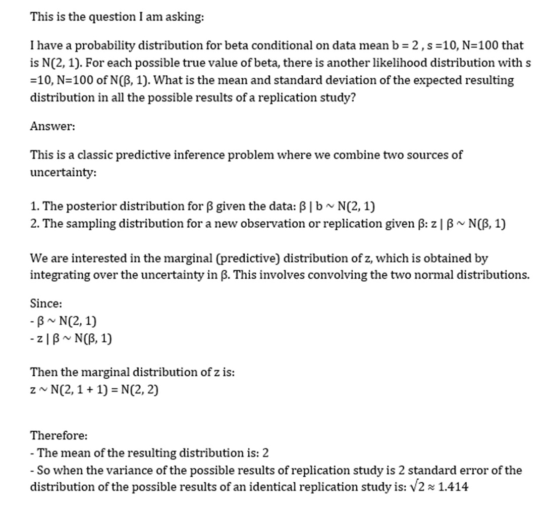
I had read the definition, which is simply: SNR = Beta / se (in the reasoning below se is standard error and s is standard deviation). In one of my example data, your approach appears to convolve N(2, 1)*N(0, 1) to give N(2, 2) whereas I convolve N(2,1)*N(2,1). In the latter situation I understand that the SNR is not relevant as N(0, 1) representing the SNR has been replaced by N(2, 1). Therefore in my reasoning below, the SNR and is not included (again I have set it out in PEG images to preserve the notation).
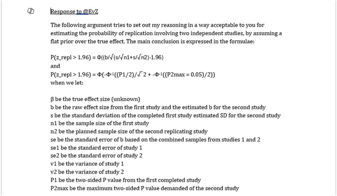
Let b be the raw effect size from the first study and the estimated b for the second study.
This is at best very imprecise. I’ll try be more precise. Let me know where you disagree!
We start with beta which is the unkown true effect. We have two studies; the “original” and the “replication” that both target beta. Let’s assume they have the same sample size n and standard deviation s. Suppose they yield estimates b and b_repl which are unbiased with the same standard error se=s/sqrt(n). In other words, conditionally on beta, b and b_repl are independent, normally distributed with mean beta and standard deviation se.
Agreed so far?
Now let’s divide everything by se. Then, conditionally on SNR=beta/se, z=b/se and z_repl=b_repl/se are independent, normally distributed with mean SNR and standard deviation 1.
Agreed?
I believe we are both interested in the conditional probability of replication, which is P(z_repl > 1.96 | z).
Agreed? Also, please note how I indicate with a vertical bar what I’m conditioning on. This is a standard practice in probability theory which you should also adopt.
Now, z and z_repl linked by their common mean, which is the SNR. This implies that to be able to evaluate (give meaning to) the expression P(z_repl > 1.96 | z) we must either assume some numerical value for SNR or some probability distribution. Now you assume that beta has the (improper) uniform distribution. Would you also assume that SNR has the (improper) uniform distribution?
Where did I omit ‘|’ in a conditional statement? My understanding is that I was not combining a noise distribution with a signal but that I am combining two signals in the form of two distributions based on data, so a SNR distribution was no longer required. I assume that beta has the (improper) prior uniform distribution (i.e. conditional on the universal set of all numbers before (i.e. ‘prior’) to any evidence, informal information or any data is available. How would some SNR change the result of my reasoning and the results of my numerical examples?
The left-hand side is a marginal (unconditional) probability. So, it’s a number between 0 and 1. The right-hand side is a function of b, s, n1 and n2. As a mathematician might say, your equality is “not even wrong”.
But now you would need to consider the joint distribution of z_repl, b, s, n1 and n2. That’s not easy! I prefer to work with P(z_repl>1.96 | z) so that I only need to specify the joint distribution of SNR, z and z_repl.
In my previous post I tried to establish a common framwork. It would be helpful if you could let me know where you agree and disagree.
(1a) Not quite. I assume that b_repl = b, s_repl = s, and if you wish for simplicity for the time being, let n1_repl = n1 and n2_repl =n2.
(2q) Agreed?
(2a) I can’t agree yet. I define z_repl differently. In order for me to understand you clearly, please give values for your SNR, z, and z_repl when, for example, b = 2, s = 10, n1=n2 = 100.
(3q) Agreed? Also, please note how I indicate with a vertical bar what I’m conditioning on. This is a standard practice in probability theory which you should also adopt.
(3a) Not quite. I am interested in P(z_repl > 1.96 | b, s, n1, n2).
I can’t agree or disagree with (3q) until I can understand where you are going until you also assume (1a) and answer my question (2a).
I apologise for not being explicit about P(z_repl > 1.96 | b, s, n1, n2), but as you imply, it was obvious what I meant because b, s, n1, n2 were on the RHS; I had copied and past P(z_repl > 1.96 | b, s, n1, n2) many times from an earlier draft and b, s, n1, n2 must have not been copied at some point and the omission perpetuated.
(4q) Would you also assume that SNR has the (improper) uniform distribution?
(4a) I can’t answer this question (4q) until you also assume (1a) and answer my question (2a). Please also display graphically your resulting distributions for beta and SNR.
We start with beta which is the unkown true effect. We have two studies; the “original” and the “replication” that both target beta. Let’s assume they have the same sample size n and standard deviation s. Suppose they yield estimates b and b_repl which are unbiased with the same standard error se=s/sqrt(n). In other words, conditionally on beta, b and b_repl are independent, normally distributed with mean beta and standard deviation se.
You answered:
I assume that b_repl = b, s_repl = s, and if you wish for simplicity for the time being, let n1_repl = n1 and n2_repl =n2.
This doesn’t make sense to me. Assuming b_repl=b means that you have two studies that yield the exact same estimates. I’m proposing that beta is the unknown true effect, while b and b_repl are two unbiased estimates from two studies. If you don’t agree with this, we’re done.
Also, you’ve just introduced 5 new symbols: s_repl, n1_repl, n1, n2_repl and n2. Let’s just assume that the two studies (original and replication) have the same same sample size which we call “n”, and the same standard deviation which we call “s”. Then the two estimates (b and b_repl) have the same standard error which we’ll call “se”.
To have a meaningful discussion, we need to agree on a common framework. So, again, I wrote:
We start with beta which is the unkown true effect. We have two studies; the “original” and the “replication” that both target beta. Let’s assume they have the same sample size n and standard deviation s. Suppose they yield estimates b and b_repl which are unbiased with the same standard error se=s/sqrt(n). In other words, conditionally on beta, b and b_repl are independent, normally distributed with mean beta and standard deviation se.
You answered:
I assume that b_repl = b, s_repl = s, and if you wish for simplicity for the time being, let n1_repl = n1 and n2_repl =n2.
This doesn’t make sense to me. Assuming b_repl=b means that you have two studies that yield the exact same estimates. I’m proposing that beta is the unknown true effect, while b and b_repl are two unbiased estimates from two studies. If you don’t want to agree with this, we’re done.
Also, can we agree (at least for now) that the two studies (original and replication) have the same sample size which we call “n”, and the same standard deviation which we call “s”. Then the two estimates (b and b_repl) have the same standard error which we’ll call “se”.