To make it explicit for you, I estimate SNR = (1.96^2*100)/10^2 = 3.48 and acknowledge uncertainty in the true effect represented by the posterior probability distribution conditional on the first study result based on a uniform distribution, and then an identical likelihood distribution for all the possible replication study results conditional on each possible true mean. The convolution of the posterior and likelihood distributions when Var_completed study = 1 gives:
There is no posterior probability without specifying a prior distribution on the SNR. And if you take the (improper) uniform distribution as your prior, then you get 0.5 instead of 0.283.
You talk about posterior, likelihood, uniform distribution, convolution but you don’t follow the rules of probability theory. I know that probability and statistics are hard, and I appreciate that you are doing your best. But I’ve put a lot of effort in explaining and at this point you’re just being stubborn.
I have explained my reasoning carefully in the pre-print and here. Your very own study supports my argument and you have been unable to explain to me in simple terms where I have gone wrong. If I was so very wrong in following the rules of probability theory, then I would have expected that you could provide an illustrative counter-example using simple data like those in my preprint and to come up with correct answers.
I find the expressions that you use to reason with me very difficult to relate to reality. For example the expression of P(z_repl > 1.96 | z=1.96) = 0.025 that you use in your arguments to provide correct answers seems to imply an infinitely large variance, which although it may be mathematically sound, does not make any sense and bears no relation to the example data that I use. Thank you anyway for taking the trouble to discuss things with me.
You write mathematical formulas as if you’ve derived them from your assumptions. But you haven’t, and you shouldn’t pretend. And to be clear: “deriving” doesn’t mean simply writing down your conclusion.
Of course, there’s no law that you have to provide mathematical derivations for your claims. Instead, you can just say: Based on my clinical experience, I’ve invented a nice formula for the probability of successful replication given the z-statistic: 1 - pnorm(1.96,z/sqrt(2),1). As it turns out, this formula works well in the context of the clinical trials of the Cochrane database. In other contexts, it may not work well.
For example the expression of P(z_repl > 1.96 | z=1.96) = 0.025 that you use in your arguments to provide correct answers seems to imply an infinitely large variance, which although it may be mathematically sound, does not make any sense and bears no relation to the example data that I use.
No, it doesn’t imply infinite variance. It just implies that we’re considering a situation where there are only null effects. Again, you’re just saying things because you can’t be bothered with actually doing the math.
I’m still going through your pre-print, but I’m getting confused by the notation. What I think is happening is there is a confusion between values on your un-standardized measurement scale with standardized Z scores under the normal density (which I’ll call the statistical scale), which can be stretched or contracted to fit an arbitrary pair of mean and variance inputs on the measurement scale.
The specific values you used map to numbers on the Standard Normal scale N(0,1) so certain calculations “work” by accident.
The numbers used in your example (especially the discussion of just 2 values) just happen to match values in the expression for a function of the Normal Density, and appear to cancel by accident.
Some of the properties with adding and subtracting standard normal deviates are: \frac{Z_1 + Z_2, + ... Z_k}{\sqrt{k}}
Summing K standard normal deviates, then dividing the sum by \sqrt{k} results in a distribution that remains Normal with a SD=1. This is a procedure to combine the information in multiple statistical tests known as the Stouffer Inverse Normal Combination Procedure.
To be fair to you, I will revisit this after reading and taking notes on your paper and being explicit in how I understand your reasoning.
I’m pretty sure Huw isn’t conditioning on all that. I think he’s only conditioning on the z-statistic of the first study. So, we just need to consider this simple set-up:
Assume some distribution for SNR. This is specific to the field of research.
z is the sum of SNR and a standard normal error e1.
z_repl is the sum of SNR and a standard normal error e2.
e1 and e2 are independent.
Huw seems to think that it follows from 2, 3 and 4 that
FWIW, I agree with your reasoning; I’m just trying to work my way through his calculations.
If he is conditioning on the Z statistic, then the naive guess for a replication study must start with the assumption that the Z stat for a replication study has a distribution N(1.96, 1).
If this is true, then I don’t see how to escape the conclusion that given that Z_{init} = 1.96 the probability Z_{rep} \ge 1.96 = 0.5, which is only a shift of the central, standard normal distribution N(0,1) to N(1.96, 1) if you don’t engage in a Bayesian analysis, even with a uniform prior, which Goodman shows does apply some shrinkage, especially for Z statistics with large deviations from 0.
That’s not quite right. Suppose we assume the (improper) uniform prior for the SNR. Then the conditional distribution of the SNR given z_init is normal with mean z_init and standard deviation 1.
Since z_repl is the sum of SNR and another standard normal error, it follows that the conditional distribution of z_repl given z_init is normal with mean z_init and standard deviation sqrt(2).
So, if we assume the (improper) uniform prior for the SNR then
Your reasoning looks superficially similar to what I was doing a few years ago when I was looking at p-value combination methods, but I wasn’t able to convince myself I was correct (because it wasn’t).
My previous thinking assumed a study with a 0 result, and then combining with the observed result using the inverse normal combination method, which shifts the observed result closer to 0.
My sticking point was assuming/retaining a unit variance, which is the basis of the methods in the book by Kulinskaya, Staudte, and Morgenthaler I mentioned in post 2. If I understand your code correctly, the variance you are inputting into that R function is = 1.4142.
RE: Shrinkage with uniform prior:
These are the results in the table from Goodman’s 1992 paper:
Probability of a statistically significant duplicate experiment
The first column (labeled mu1=mu2) is the so-called post hoc power. That means making the (false!) assumption that the SNR is equal to z_init. Then the conditional distribution of z_repl given z_init is normal with mean z_init and standard deviation 1.
A two-sided p-value of 0.1 corresponds to z_init=1.64. In that case, the post hoc power is 1 - pnorm(1.96,1.64,1)=0.37. That is the first entry of the first column (mu1=mu2).
If we assume the (improper) uniform prior for the SNR, we get
How would you describe the results in the table after 0.03, where the uniform prior reduces the replication probability, which continues until the end of the table?
There’s no shrinkage in the sense that that 1.64 appears in both calculations.
The uniform prior means there’s less information in z_init about the SNR compared to assuming that the SNR is equal to z_init. So small p-values provide less evidence for successful replication.
I understand that, and it makes perfect sense. My confusion is why is it incorrect to say that the replication probability estimates are shrunk, since the increased variance in the calculations seems to be pulling extreme p values in the data closer to the center of a uniform distribution with a range between 0 and 1?
Addendum: In response to @EvZvery patient and helpful reply (LaTeX added by me for readability):
I follow all of this reasoning so far, particularly the estimator has a distribution N(\beta,1).
I can see your point now; you were working on the Z scale, and I was thinking of how the probabilities under the uniform prior assumption change relative to the (false) assumption that the initial estimate equals the true SNR.
I guess my confusion was that I (previously) didn’t understand how to get the posterior variance, when the distribution of multiple Z scores is N(\beta,1) It looks to me that the posterior standard deviation in your R code:
Note: A definition of the R function “pnorm” can be found here:
As \sqrt{2} = 1.4142, the Bayesian answer must have greater uncertainty than simply conditioning on the observed estimate, which is distributed as N(\beta,1) as assumed above.
Relating this back to inverse normal combination methods – the posterior standard deviation under the uniform prior assumption of the SNR is analogus to a Stouffer inverse variance combination method where the posterior standard deviation is \sqrt{1+1} = \sqrt{2} = 1.4142
Just to remind you of my notation: Let beta denote the (unobserved) true effect effect of the treatment and let b be a normally distributed estimator with mean beta and (known) standard error s. Define the z-statistic z=b/s and the signal-to-noise ratio SNR=beta/s. The z-statistic then has the normal distribution with mean SNR and standard deviation 1. So, you can think of z as an unbiased estimator of SNR.
Now, if we assume a normal prior for the SNR with mean zero and standard deviation sigma, then the posterior mean of the SNR is
E(SNR | z) = z*sigma^2/(sigma^2+1).
sigma^2/(sigma^2+1) is the called the shrinkage factor. If sigma becomes very large, so that the normal distribution approaches the uniform, then you can see that the shrinkage converges to 1. In other words, if we assume the uniform prior then E(SNR | z)=z. No shrinkage.
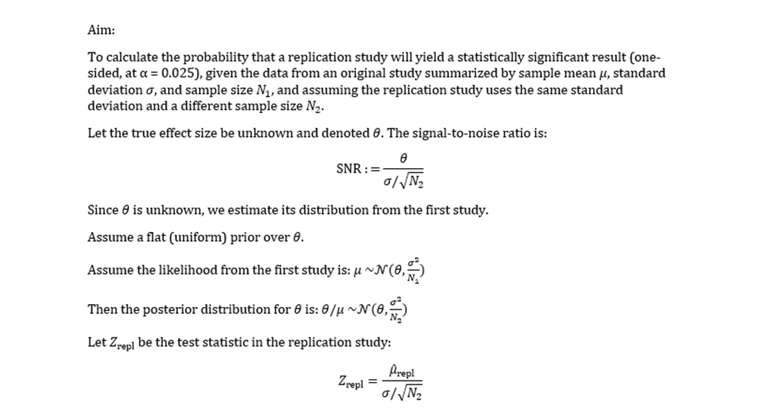
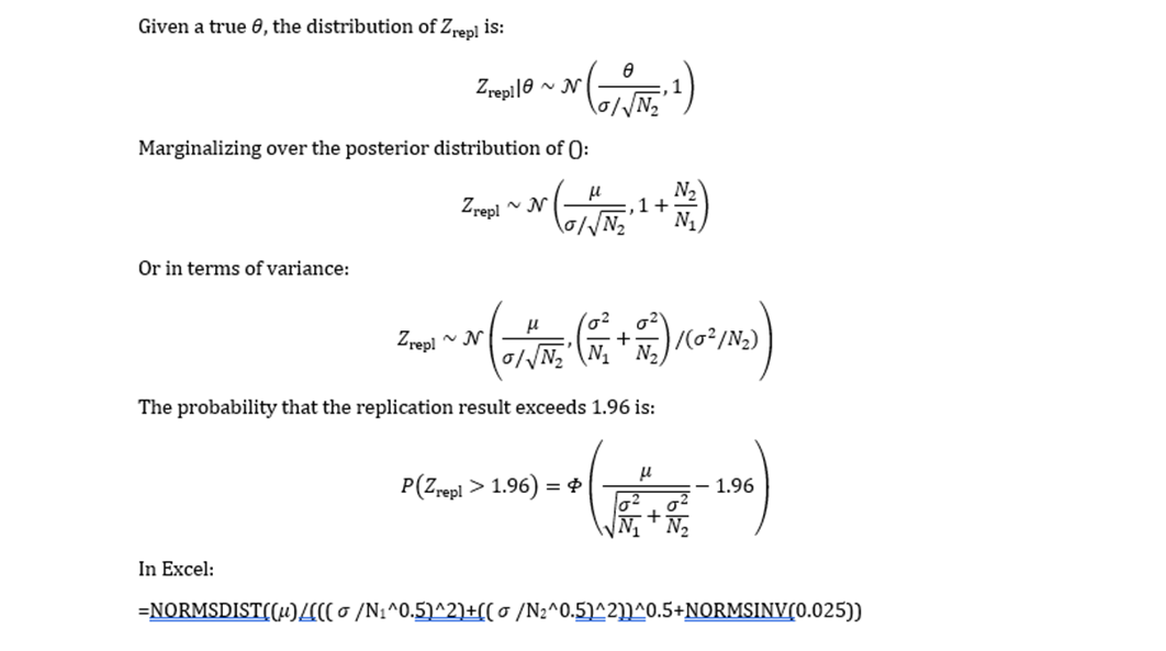
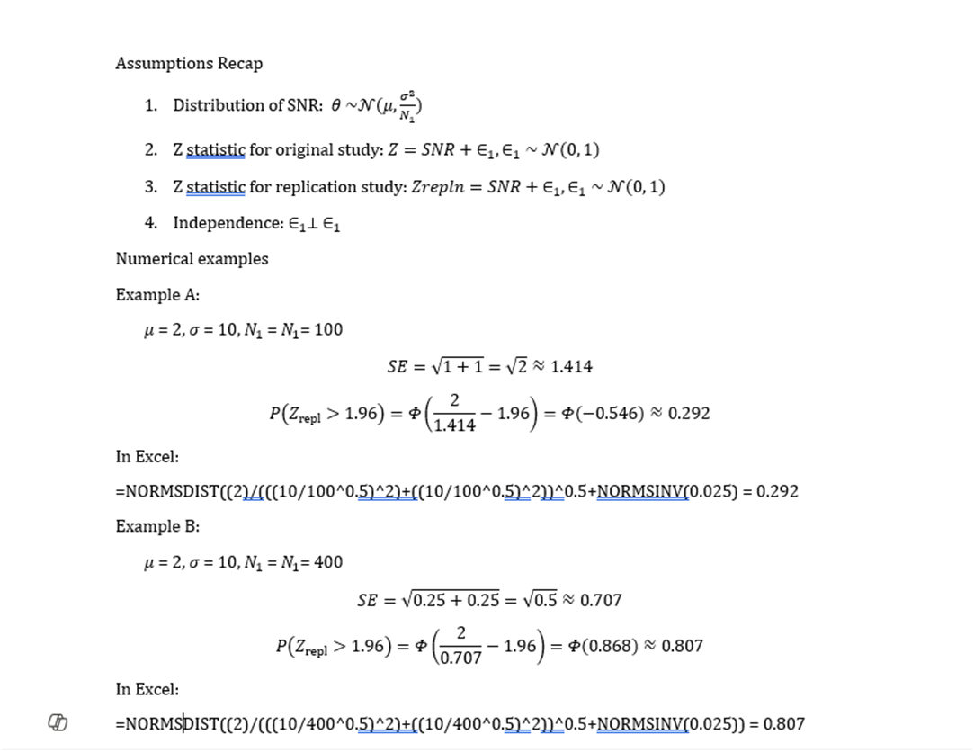
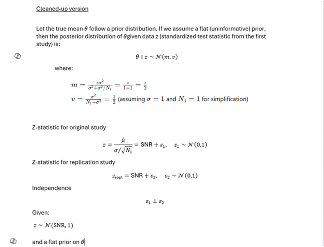
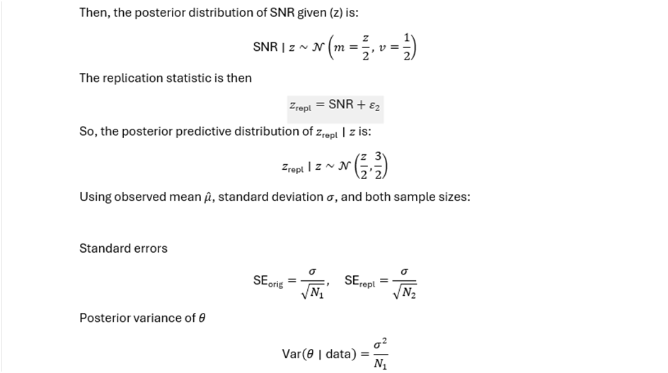
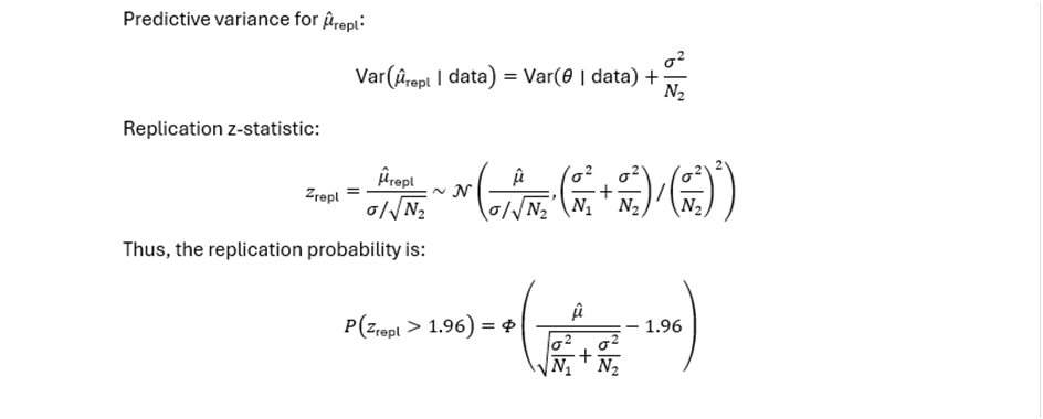
I have tried to explain myself here using mathematical notation to try to help you @EvZ and @R_cubed to follow my reasoning. In order to preserve the format, have used JPEG images.
I have been concerned since my students days about the misunderstanding about statistics in those who were not taught it as their first degree or as a major part of it. I was intrigued to read David Spiegelhalter state in a recent book of his (Spiegelhalter D. The art of statistics. Learning from data. Penguin Random House, 2019). that “learning from data is a bit of a mess” and how students are baffled by statsitics, especially P values. I have a feeling that much of this is due to problems in pinning down the concept of prior probability. I address this in my recent preprint (https://arxiv.org/pdf/2403.16906) and try to show that such a focus may be able to provide a lot of insight into the reasons for the replication crisis.
I appreciate the effort, but you’ll need to clean up your notation for me to be able to understand. You use mu both for the likelihood of the first study and for the mean of the distribution of the SNR. You write also theta/mu for the ppsterior distribution and mu-hat_repl for the estimate in the replication study. You also use sigma in multiple meanings.
It’s easiest to assume N1=N2 and to keep to the following description.
Assume a normal distribution for the SNR with mean mu and standard deviation sigma.
z is the sum of SNR and a standard normal error e1. So, z ~ N(SNR,1)
z_repl is the sum of SNR and a standard normal error e2. So, z_repl ~ N(SNR,1)
e1 and e2 are independent.
You can think of this as the special case where the SEM in both studies is 1 (but it’s actually more general). To make things even easier I recommend you assume mu=0. You will then find that the conditional (or posterior) distribution of the SNR given z is again normal with mean
m = z*sigma^2/(sigma^2 + 1)
and variance
v=sigma^2/(sigma^2 + 1)
Since z_repl is the sum of the SNR and a standard normal error, it follows that the conditional distribution of z_repl given z is normal with mean m and variance v+1.
If you assume the flat prior (i.e. sigma is extremely large) then the conditional distribution of z_repl given z is normal with mean z and variance 2.
You should really say what the symbols mean, but I think I understand. Is theta the true effect? And is sigma/sqrt(N1) the standard error of the estimate from the first study? And are you assuming that sigma/sqrt(N1)=1?
If that’s the case, then theta is what I call signal-to-noise ratio (SNR) and
z | theta ~ N(theta,1).
If theta has the (improper) uniform distribution, then the conditional (posterior) mean of theta is not z/2 but z. And the conditional variance of theta is not 1/2 but 1.