Some thoughts on uniform prior probabilities when estimating P values and confidence intervals

Well my understanding is that there are two types of prior. The first is the so-called ‘unconditional prior’ that is actually conditional on a universal set, the latter being essential when applying Bayes rule.. A Bayesian prior is conditional also on prior knowledge of the study or other additional information such as the SNR. My understanding is that Kass (1990) is addressing other such ‘conditional prior’ information.

Now it sees to me a matter of judgement as to how or when to incorporate such other prior knowledge and their ‘conditional prior’ probabilities into a calculation. In my case I only assume a flat prior and Gaussian distributions but no other ‘conditional prior’ in my expression, the calculations being conditional only on b, s, n1 and n2.

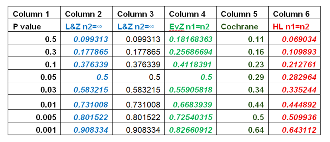
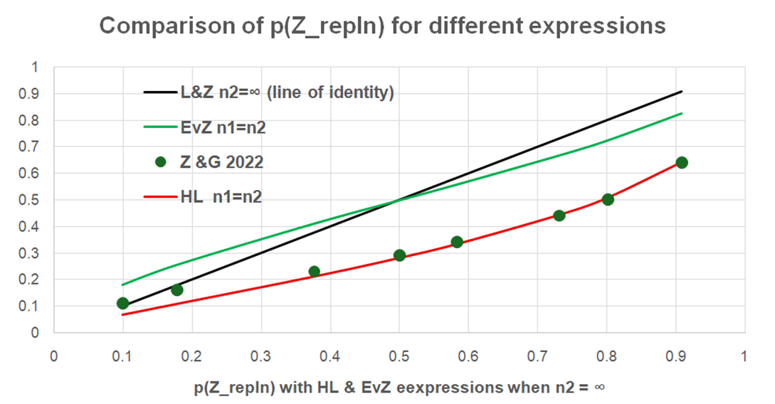
P(Z_{\text{repln}} > 1.96 \mid b, s, n_1, n_2) = \Phi\left( \frac{b}{\sqrt{\left( \frac{s}{\sqrt{n_1}} \right)^2 + \left( \frac{s}{\sqrt{n_2}} \right)^2}} - 1.96 \right)

It is also my understanding that there are no right or wrong opinions, but only those that have been justified logically based on clear facts and assumptions and those that have not.

None of this phrasing is standard in the probability or statistics literature, but if I charitably interpret your meaning, you want to retain a state of uncertainty about the validity of the first estimate (converted to a Z score). This is already done if you assume normality, as your standard deviation, as a standard normal deviate is known to have a variance of \pm 1

This desire to discount the first estimate isn’t unreasonable, but your mathematical representation of this isn’t correct. You can think of the mathematical modelling of a statistical experiment like a U.S. Congressional investigation. Two questions are asked of witnesses:

  1. What do you know?
  2. When did you know it?

Your representation amounts to ignoring your first estimate and your assumption that the errors are normal as if you never had it, then re-introducing it ex-nihilo.

A “non-informative” prior over \mathbb{R} maximizes the weight in the data, but produces a proper probability distribution when the likelihood is normal. There are other cases as the paper by Robert Kass discusses, but just understanding how this works for the normal model is important now.

FWIW, I had to search for these results related to uniform priors in order to understand how EwZ derived his R code.

If you are going to compute anything sensible, I can’t see any way of avoiding the assumption that the 2 estimates come from the same normal distribution. In order to compute any measure of distance or closeness between 2 estimates for prediction, you need to condition on something - ie. assume a certain mean value of a normal distribution.

In the calculation I estimate p(Beta_i | b) for all i based on v1 calculated from s and n1. This gives all the probability distribution of all possible values of Beta_i conditional on b in very many repeat studies. Then for each Beta_i for each possible repeat study, I estimate the likelihood of b_rep conditional on each possible Beta_i based on v2 from s and n2. The net result of this operation is p(b_repln_ j | b), the distribution being based on v1 + v2.

W

You are going to have to show the parameter values you use for the uniform distribution in your calculation, even though I strenuously object to using a uniform prior for the second study, after you have seen the first.

Specifically, I want to see your assumptions and how you mathematically represent your epistemic state:

  1. Before the first study
  2. After the first study, but before the second.

How does the first study change your epistemic state, represented as a probability distribution?

The beauty of Bayes Theorem is that it is an elegant way to represent learning; the prior for 1 experiment is updated by the data to form the posterior, which can then be used as a prior for the next experiment.

It would be very helpful if you structured your thoughts like a proof, so the rest of us can follow your reasoning. It doesn’t have to be perfect, but it would make things much easier. If you have to look up mathematical justifications, go ahead. I do it all the time before posting.

As an example, this is valuable for clarifying the logic of any mathematical argument.

Why do you think this? I used a flat prior to estimate the posterior p(Beta_i |b). This becomes the conditional prior to combine with each likelihood p(b_repln_j | Beta_i). The results in p(Beta_j | b), the distribution for the latter having a variance of v1+v2.

I object to it because it makes no mathematical sense, from either a Bayesian or a Frequentist point of view.

I don’t use the flat prior twice. Explain where you think that I do this.

You use the flat prior before the second study, totally ignoring the data in the first, yet you want to use it somehow for prediction. That makes no sense.

The (improper) uniform prior, if it is to go anywhere, should be asserted before the first study. Then following the logic of Kass, the posterior is merely translated linearly from the assumed sampling model N(0,1), with a posterior of N(\theta, 2), It is from there you start computing predictions for the second study.

What I am doing is a short chain of conditional probabilities. So does this help you?:

Posterior on the True Effect:

P(\beta \mid b, s, n_1, U) \sim \mathcal{N}\left(b,\ \frac{s^2}{n_1} \right)

Sampling Distribution of Replication Estimate:

P(b_{\text{repl}} \mid \beta, s, n_2, U) \sim \mathcal{N}\left(\beta,\ \frac{s^2}{n_2} \right)

Convolution of the Two Distributions:

P(b_{\text{repl}} \mid b, s, n_1, n_2, U) \sim \mathcal{N}\left( b,\ \frac{s^2}{n_1} + \frac{s^2}{n_2} \right)

Standardized Replication Z-Score:

z_{\text{repl}} = \frac{b_{\text{repl}}}{\frac{s}{\sqrt{n_2}}}

Predictive Probability of Replication Success:

P(z_{\text{repl}} > 1.96 \mid b, s, n_1, n_2) = \Phi\left( \frac{b}{\sqrt{\frac{s^2}{n_1} + \frac{s^2}{n_2}}} - 1.96 \right)

RE: “Posterior of the True Effect” is obscure when stated before any assumptions about the prior and likelihood. It follows from combining the prior and likelihood according to Bayes Theorem.

In a decision theory set up, you have:

  1. a state space (called the State of Nature) or parameter space,
  2. a sample space (conditional on some parameter),
  3. some sort of cost function, and
  4. a prior on the states of nature.

The goal is to develop methods such that the difference between Posterior (or the estimator) and the state of nature approaches zero as the sample size increases. We would also like this difference to approach zero as quickly as possible.

Frequentist methods can be replicated in a Bayesian framework with various concepts of “non-informative” or “least favorable” priors, which are better thought of as priors that maximize the weight of the data or minimize the maximum loss, and result in proper probability distributions.

I have no idea what U refers to in your notation. If it refers to the Uniform distribution, you need to report what parameters you are using. As it stands now, your use of different probability distributions on each side of the \sim operator looks incorrect to me.

U represents the universal set of all numbers in this case. The flat uniform prior is conditional on U. A universal set is an essential part of Bayes rule.

This is not how to formulate a mathematical argument. You must specify precisely what set of numbers you are talking about. Then we know what algebraic laws apply.

In your notation, it was not clear if you were referring to a set or a distribution. That matters, and it makes it hard for people with mathematical training to parse your arguments and seriously consider them.

I’ll give you a hint: you probably want to specify the real number system \mathbb{R}.

Thank you for that suggestion.

This is wrong because you keep . making . the . same . mistake. Please try to follow the correct derivation:

P(z_\text{repl} > 1.96 \mid b,s,n_1,n_2) = P(b_\text{repl} > 1.96\frac{s}{\sqrt{n_2}} \mid b,s,n_1,n_2)
=P\left(\frac{b_\text{repl} - b}{\sqrt{\frac{s^2}{n_1} + \frac{s^2}{n_2}}} > \frac{1.96\frac{s}{\sqrt{n_2}} - b}{\sqrt{\frac{s^2}{n_1} + \frac{s^2}{n_2}}} \mid b,s,n_1,n_2 \right)
=P\left(\frac{b - b_\text{repl}}{\sqrt{\frac{s^2}{n_1} + \frac{s^2}{n_2}}} < \frac{b - 1.96\frac{s}{\sqrt{n_2}}}{\sqrt{\frac{s^2}{n_1} + \frac{s^2}{n_2}}} \mid b,s,n_1,n_2 \right)
= \Phi\left( \frac{b - 1.96\frac{s}{\sqrt{n_2}}}{\sqrt{\frac{s^2}{n_1} + \frac{s^2}{n_2}}} \right)

The second equality is the usual standardization of b_\text{repl} by subtracting the (conditional) mean and dividing by the (conditional) standard deviation.

If s^2/n_1 = s^2/n_2=1 then this simplifies to \Phi\left( \frac{b - 1.96}{\sqrt{2}} \right) instead of your mistaken \Phi\left( \frac{b}{\sqrt{2}} - 1.96 \right).

1 Like

What we are doing of course is trying to derive mathematical models to predict the result of a natural process, which is always difficult (like medical prognosis). When n2 = ∞, then both EvZ and HL expressions give the same probability of replication. For example in your two simplified examples, when n2 = ∞, instead of √2 in the denominators we would get √1 and EvZ and HL expressions give the same result of ɸ(b/1-1.96). A difference happens when n1<<∞ and n2<<∞ and when n1=n2 or when n1≠n2.
Table 1


Columns 2 to 6 of Table 1 show the probabilities of replication for different P-values from P=0.5 to P=0.001 as laid out in Column 1. The probability of replication for both methods HL and EvZ are in Columns 2 and 3 when n2 = ∞. Column 4 shows the probabilities of replication using the EvZ expression when n1=n2. Column 5 (Cochrane) shows the probabilities of replication arising from the Cochrane data as described in van Zwet, E. W., & Goodman, S. N. (2022) (see (link) in post number 50). Column 6 sets out the probabilities arising from HL’s expression when n1=n2

Figure 1

Figure 1 is a plot of the data in Column 2 (on the horizontal axis) against columns 3 to 6. The horizontal scale is the probability of replication for both methods HL and EvZ in Columns 2 and 3 when n2 = ∞. The black line is of identity when the expected probability of replication in a second study conditional on the P value based on n2 = ∞. The large green points are the probabilities of replication conditional on the P value based on the Cochrane data. The red line is the probability of replication conditional on the P value based on HL’s expression; this predicts very well the Cochrane probabilities of replication. The green line represents the probabilities of replication conditional on each P value based on EvZ’s expression. The latter overestimates the Cochrane results and is very close to the line of identity. It also predicts that when P>0.05 and n1=n2<< , the probability of replication is greater than when N2 = , which does not make sense. Therefore HL’s approximation appears to give plausible predictions of replication whereas that of EvZ does not. What is you explanation for this? Am I mistaken in any way? If so how?

OK, this is completely useless. You seem to be incapable of understanding that you’re making a high school level math mistake. All you need to do is follow the simple derivation in my last post to see that from your own assumptions (stated in your post 169) you don’t get your conclusion (last line of your post 169).

Please explain the above and also why your derivation creates actual results that appear to make no sense.

You are taxing my time and patience, but I’ll give it one more try. In your post 169 you assume the flat prior and conclude

I don’t fully agree with your notation, but I agree with what you mean. Now, you claim that this implies

P(z_\text{repl} > 1.96 \mid b,s,n_1,n_2) = \Phi\left( \frac{b}{\sqrt{\frac{s^2}{n_1} + \frac{s^2}{n_2}}} - 1.96\right).

This implication is simply false. It’s just a math mistake. Using your notation, and taking only baby steps, the correct implication is:

P(z_\text{repl} > 1.96 \mid b,s,n_1,n_2)

=P(b_\text{repl} > 1.96\frac{s}{\sqrt{n_2}} \mid b,s,n_1,n_2)
=P\left(\frac{b_\text{repl} - b}{\sqrt{\frac{s^2}{n_1} + \frac{s^2}{n_2}}} > \frac{1.96\frac{s}{\sqrt{n_2}} - b}{\sqrt{\frac{s^2}{n_1} + \frac{s^2}{n_2}}} \mid b,s,n_1,n_2 \right)
=P\left(\frac{b - b_\text{repl}}{\sqrt{\frac{s^2}{n_1} + \frac{s^2}{n_2}}} < \frac{b - 1.96\frac{s}{\sqrt{n_2}}}{\sqrt{\frac{s^2}{n_1} + \frac{s^2}{n_2}}} \mid b,s,n_1,n_2 \right)
= \Phi\left( \frac{b - 1.96\frac{s}{\sqrt{n_2}}}{\sqrt{\frac{s^2}{n_1} + \frac{s^2}{n_2}}} \right).

This is a very basic derivation that any high schooler or first year student should be able to follow.

Notice how in the second equality I subtract the (conditional) mean b and divide by the (conditional) standard deviation \sqrt{\frac{s^2}{n_1} + \frac{s^2}{n_2}} of b_\text{repl}. That is called standardization.

Can you follow each of the 4 steps? Make sure you understand! If the steps continue to “make no sense” to you, then you really should not be trying to write papers about statistical methodology.

Of course I can follow your 4 steps and you jolly well know that I can. I have emphasised already that I have no problems with your maths (e.g. see post 145); I know exactly how your derivation was arrived at. It is our concepts of the process of replication that is different, leading to different assumptions and a different model for the probability of replication.

My concepts and intuition are based on my experience of replication in practice when actually working as diagnostician, decision maker, researcher and dealing with the latter’s consequences in medical practice and research. I always try to express my understanding in terms of mathematical modelling, testing my mathematical expressions using real data on Excel (as I showed you in my recent post 175).

So please understand, the issue is not the maths but the assumptions made when constructing the mathematical model and testing it on real data

So please understand, the issue is not the maths but the assumptions made when constructing the mathematical model and testing it on real data

Your assumptions don’t imply your conlusion. That doesn’t strike you as problematic?

If your “intuition” doesn’t agree with the conclusion from your assumptions, then you should change your assumptions, not your conclusion.

Of course I can follow your 4 steps and you jolly well know that I can.

So then claiming a conclusion that doesn’t follow from your assumptions is intentionally misleading. Nice.