We require all users to include their real first and last names in their profiles. Please fix your profile to remain on the system.
1 Like
I was wondering if you have any recommendations in settings where you want to sequentially evaluate the added value of multiple predictors.
Take for example the following situation. We have a core set of routinely measured predictors and want to evaluate the added value of several other predictors. Some of them are comparatively cheap or easier to measure (e.g. liver enzymes), others are more expensive (e.g. genes). You could evaluate the added value of all these candidate predictors against the core model, but this would be rather senseless if the cheaper candidate predictor already improves the model substantially. Example, we have the following models:
- M1: Core model
- M2: Core model + cheap predictor 1
- M3: Core model + cheap predictor 2
- M4: Core model + expensive predictor 1
- M5: Core model + expensive predictor 2
We compare the added value of all four predictors against the core model and find that cheap predictor 2 improves the model (let’s say it adds more than 10% new information), but so does expensive predictor 1. However, if you would evaluate the added value of expensive predictor 1 against a model that included cheap predictor 2 then it would add almost no new information. So:
- Mnew 1: Core + cheap predictor 2
- Mnew 2: Core + cheap predictor 2 + expensive predictor 1
Here, expensive predictor 1 contributed almost no new information.
In particular, what I was wondering in a setting such as this:
- How would you define sufficient added information for determining whether a predictor adds enough information to warrant inclusion in a new, updated model? I’m thinking that setting strict boundaries (e.g. always has to add 10% new information) would be trivial (and lead to similar issues as variable selection based on p-values) and so this process will probably always be somewhat subjective and should be weighed against other concerns such cost/availability of the predictor.
- Also, in this setting to some extent you are performing variable selection although in a much more directed/informed manner than ‘simple’ stepwise procedures. Should then this entire process be re-evaluated in an internal validation procedure or would it be acceptable to calculate the added value/information from optimism-corrected estimates of model performance?
I’m asking because I am currently dealing with a situation such as this one and am a little unsure how to proceed. Briefly, I am working on the prediction of a continuous outcome for which several models already exist. However, all of these have been constructed through automated variable selection procedures. As a result, they all contain one or more predictors that are not routinely measured (e.g. due to lack of an indication or constraints in time or cost required for their measurement) or that are complex to use (e.g. phenotypes that are themselves constructed/calculated from the measurement of several other variables).
So I compiled a core set of routinely measured predictors from the existing literature and want to assess the added value of the other candidate predictors on top of this. If they add enough information, this might warrant their measurement.
All these other predictors I organized according to their availability and/or estimated cost for measuring them and how frequently they feature in existing models. Together, I have about 20 candidate predictors of which to assess the added value. A few of these are reasonably cheap, though not routinely measured, and add a decent amount of information; 33% as estimated from:
1 - (R^2_{core}/R^2_{core+\text{cheap predictor}})
I calculated this from the optimism-corrected estimates of the R2 of both models. The other 15+ remaining ones add almost nothing on top of this (around 2% added information if you add them all against the model that included the cheap predictors).
At this point, I got caught up in some doubts about my concerns above so any advice is greatly appreciated!
2 Likes
This is a really good problem to discuss. To start with the “data mining” part of the question, not a lot of work has been done on quantifying added predictive information when variable selection has been done. In general, variable selection is a bad idea so it’s hard to get very motivated to develop a method that handles that, although bootstrapping as you mentioned sounds very reasonable. But I would start with “chunk tests”. Before looking individually at “cheap 1” “cheap 2” etc. I’d have a model with both “cheap” variables and a model with both “expensive” variables, to quantify the overall added value of “expensive”. But then go back to the context and treat the 20 candidate predictors as a set, with at least 20 d.f. Supplement this with a bootstrap confidence interval for the rank of each of the 20, ranking on the basis of improvement in -2 log likelihood (i.e., in terms of the likelihood ratio \chi^2 test for each predictor). This takes into account multiplicity and the difficulty of the task.
Any time you can compute the actual cost of a predictor you can sort the predictors by increasing cost and plot model likelihood ratio \chi^2 as a function of cost. Then you are no longer doing any dangerous variable selection as the ordering of predictors is pre-specified, and you can pick the “best bang for the buck”.
5 Likes
Thank you for your advice! I’m going to try this out, but before I start I wanted to make sure I’ve got the details right.
I’m also not particularly fond of blind/automated variable selection, which is also what inspired this project after reading your blog post. We wanted to see if the five routinely measured predictors out of the (over) 20 that are used in various models would suffice and if the others would actually add anything on top of them. But then as I started out I realized this was basically turning into variable selection through added value.
Did I understand correctly that you meant:
- Core + all ‘cheap’
- Core + all ‘expensive’
I was planning to do of a version of this already. For some more details, I have a reasonable idea about the relative costs/availability of the remaining predictors and roughly ordered them based on this and how often they have featured in the existing models:
- Low (additional) cost or even reasonably available, infrequently featured in existing models
- Moderate (additional) cost, frequently featured in existing models
- Moderate or high (additional) cost, infrequently featured in existing models
Beforehand, my plan was to evaluate the added value of each of these sets on top of the core five predictors, mostly to rule out situations where for example five low-cost predictors together provide a decent amount of information but the individual ones don’t. But then I started wondering how to deal with these comparisons once a ‘cheaper’ predictor already provides a lot of information.
For the ranking analysis and the plots of model likelihood ratio X^2, you mean I should use the partial X^2 such as you use for ranking in section 5.4 of your RMS book I think, correct? Assuming so, I produced the plots and attached them here for others who are interested. I color-coded the predictors, black being the core five, blue the low-cost, yellow the medium-cost and red the high-cost ones.
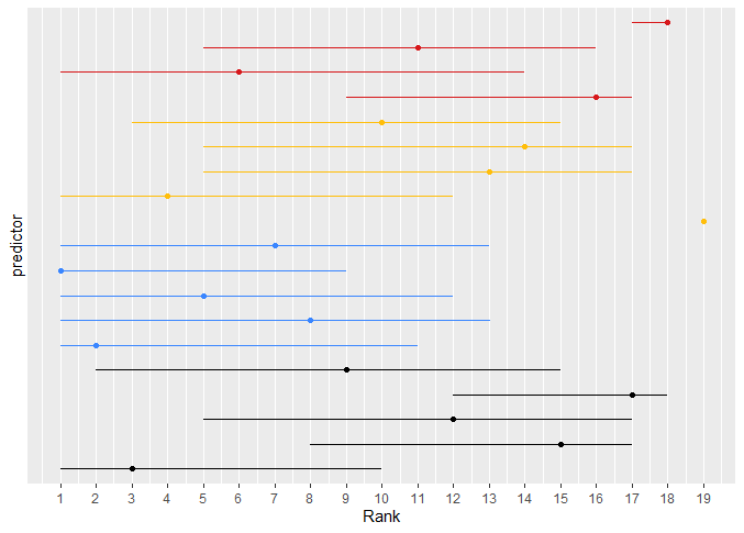
As you discussed for your example in the book, the CIs are very wide. The ‘core’ predictors seem to be somewhat in the middle to upper-middle ranks and also feature a reasonable improvement in -2 log likelihood. The yellow one that consistently ranked high was the one predictor I mentioned in my previous post that resulted in 33% or so added information.
4 Likes
What a beautiful analysis. I think you’ve done all the steps extremely well. I plan to link to this post from my course materials. I think that the results are clear only for the predictor at the top in the left panel, otherwise there is not enough information to make choices of predictors.
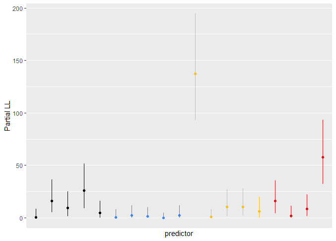
Nice! I’m working on a similar analysis. To me it seemed more informative to rank order variables by the partial Chi-squared but then to display the partial Chi-squared quantity on an axis. Turned out like a bar graph with some whiskers for confidence intervals. That way it was clear that some predictors were not just consistently ranked higher than others, but that the magnitude of additional predictive information was huge.
4 Likes
That is a really nice suggestion too! If I have some spare time I’ll try this out and post it, but I might try ordering them within each category of cost/availability in my case (because I have quite a clear idea which ones would be more available or might take more effort to measure, time or money-wise). I guess it will turn out sort of like a marriage of the two images above, so the y-axis from the second with everything ordered according to the point estimates of the rank on the x-axis from the first?
The only potential downside I’m thinking might be that for many predictors the rank is quite unstable as you can see in the examples in the RMS book. I’m thinking that unless you have some (strong) independent predictors, you might end up concluding that some variables are consistently ranked higher while this is quite variable.
And less useful if there are no impressive differences to show. Still informative to show that the existing differences are small and nothing to write home about.
1 Like
If you can rank on the basis of data collection cost you can show the cumulative model likelihood ratio \chi^2 as you add variables and instability largely goes away. Instead of \chi^2 you can also plot \chi^{2} - kp for degrees of freedom p. k = 0, 1, 2 respectively for unpenalized \chi^2, penalized for chance association, or penalized for overfitting (AIC).
1 Like
Dear Professor Harrell,
Firstly, thank you for again producing high-quality, accessible learning material. I find the blog posts and the BBR course easy to follow (even being a physicist and not a statistician)!
I have a question I would like to discuss which may relate to other discussions on this forum – so hopefully not a silly one.
In the below scenario, the accepted model represents routinely measured predictors, and we are working with a time-to-event outcome. The example shows two sets of predictors (1 and 2). I want to evaluate which set improves the model, but do not want both ‘predictors 1’ and ‘predictors 2’ (as the main question is related to which method of obtaining the predictors leads to better model performance).
- Accepted model
- Accepted model + {predictors 1}
- Accepted model + {predictors 2}
From my understanding – I can perform an LR test to assess 2 vs 1, and 3 vs 1. This will have more sensitivity than the commonly reported approach (comparing c-indices).
However, I want to re-evaluate the process using internal validation (cross-validation or bootstrap resampling). I have experience seeing c-index reported in this scenario (typically papers reporting the average value with confidence intervals). I know you mentioned in a reply above that with an LR test you may not need cross-validation, so in this scenario would we instead concentrate on optimism-corrected versions of other statistics reported in this blog post or could we still perform a similar test?
Thank you in advance,
Angie.
2 Likes
Super question Angie. The c-index is not sensitive enough to use for such comparisons, and as you stated you have to go to a lot of trouble to de-bias it using resampling methods. The log-likelihood provides optimal assessments and accounts for the number of opportunities (parameters) that you give a set of variables to be predictive.
As your models are not nested, the usual LR test doesn’t apply, as you noted. The maximum likelihood chapter in the RMS book covers (and the blog article briefly mentions) the adequacy index, and you can get a real LR test by comparing models to a “supermodel” that you are not really interested in. For your case, the supermodel has the accepted variables + predictors 1 + predictors 2. Compare your model 2. with this supermodel to see if predictors 2 add to predictors 1. And do the reverse. You can compare the resulting two LR statistics to ask the question of whether predictors 1 add more to predictors 2 than predictors 2 add to predictors 1. This indirectly answers your real question.
This approach tells you whether either model is adequate. It is possible that you really need to combine the models.
You can also use relative explained variation as detailed in the blog article.
4 Likes
Thank you for the great response Prof. Harrell.
I really like the idea of using adequacy index/relative explained variation – it feels much more intuitive than the c-index and even stronger alongside comparison to the ‘supermodel’. I will definitely be implementing these comparisons and sharing this post.
I did have a follow-up question for further understanding. If we used adequacy index as our model comparison metric, would it also be appropriate to use this same measure on external data (i.e. model AB and model A fitted without change to new data)? I know for c-index you can use survest and rcorr.cens in the rms package for performance. I was wondering whether something similar for adequacy index could work, or if it is more appropriate to stick with c-index and calibration in the ‘validation’ context? I assume these are asking different questions i.e. how does the cox-model perform on new data (c-index) and does the improvement in model performance remain on new data (AI)?
Thank you again for the help and apologies for any misunderstanding.
Hi Angela - The log-likelihood is the gold standard whether referring to training data or test data. For test data this is the out-of-sample log-likelihood which just means that in its computation the regression coefficients are frozen at their training data estimates. The R rms package computes this somewhere but a quick approximation to it is to form the linear predictor X\hat{\beta} from X_{new} and \hat{\beta}_{old} and run a new model on the new data using this as the sole variable. This will give you the right answer except that the slope of the linear predictor (which is a pretty good measure of calibration accuracy here) should have been fixed at 1.0 for an unbiased evaluation.
2 Likes
Hello! Could you please provide a code snippet of how you’d achieved this plot. R is not my primary language and I am struggling to create the plot.
1 Like
Dear prof. Harrell,
thank you for your post. I read it thoroughly and reproduced most of the code in Python.
However, I have questions regarding feature selection in the model.
- Should we include new predictors with the largest values from multiple LLR tests?
- Should the predictors with negative Chi-squared be included?
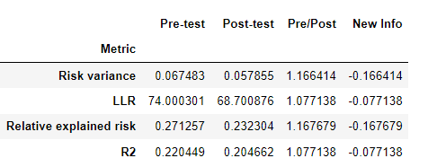
- I’ve also measured difference between LLRs for two models, but predictor was higher, resulting in lower Log Likelihood gain of full parameter model.
|Metric                   |  Pre-test | Post-test | Pre/Post |  New Info |
|:-----------------------:|:---------:|:---------:|:--------:|:---------:|
| Risk variance           | 0.051789  | 0.053781  | 0.962963 | 0.037037  |
| LLR                     | 78.966431 | 65.819788 | 1.199737 | -0.199737 |
| Relative explained risk | 0.207186  | 0.215990  | 0.959239 | 0.040761  |
| R2                      | 0.156520  | 0.195353  | 0.801216 | 0.198784  |
Should I include the predictor? Should I take the absolute difference of LLRs?
Feature selection is not a good idea in general. It’s best to either
- pre-specify the model and stick to it, or
- pre-specify a penalization function and use that
The blog post is intended for the comparison of two or three models. Stepwise variable selection has disastrous performance, even worse when collinearities exist.
1 Like
Thank you for your response. However, when I use pre-specified model and compare only one added predictor it results in a decrease in performance - every “new information” metric mentioned in the article was negative.
Therefore, I decided to make the model less complex and choose most important parameters based on Boruta algorithm A Statistical Method for Determining Importance of Variables in an Information System | SpringerLink, so that added information metrics would remain positive.
What happened with the gold standard metric (log-likelihood)? If it got worse then there is a programming problem.
Not only Log Likelihood got worse, but all metrics showed in the article:
Based on the formula:
![]()
Likelihood ratio may be negative if the new model has a lower log-likelihood than the present model. That’s what I observe in my fit.
Given the use of the same sample of observations throughout, the log likelihood must get lower when you add a new predictor, and the LLR \chi^2 statistic being -2 \times that plus a constant must get larger. So there is a programming problem. You’ll find this easier to do in R. At any rate, run it parallel in R to check Python code.