How to infer the analysts' priors from this figure?

[davidcnorrismd]

Here is Figure 1B from Fourie Zerkelbach &al (2021) [1].

In the text, it is presented as evidence for a “bell-shaped” exposure-response relationship:

No doubt the modeling here was done in a frequentist framework (if any), but it seems to me that a Bayesian view can be adopted here, in which we ask what priors would have yielded the curves as drawn, under a reasonable Bayesian model. Here ‘reasonable’ would impose a certain amount of smoothness; this could become the parameter of a family of priors. Presumably the tails (and even the negative probabilities plotted) offer useful information about the prior outside the range of the data.

How would people be inclined to go about this, technically? Might there even be a somewhat standard or customary — dare I say, ‘obvious’? — approach to reverse-engineering this prior?

---

1. Fourie Zirkelbach, Jeanne, Mirat Shah, Jonathon Vallejo, Joyce Cheng, Amal Ayyoub, Jiang Liu, Rachel Hudson, et al. Improving Dose-Optimization Processes Used in Oncology Drug Development to Minimize Toxicity and Maximize Benefit to Patients. Journal of Clinical Oncology, September 12, 2022, JCO.22.00371. https://doi.org/10.1200/JCO.22.00371.

[R_cubed]

Blockquote
No doubt the modeling here was done in a frequentist framework (if any), but it seems to me that a Bayesian view can be adopted here, in which we ask what priors would have yielded the curves as drawn, under a reasonable Bayesian model. Here ‘reasonable’ would impose a certain amount of smoothness; this could become the parameter of a family of priors. Presumably the tails (and even the negative probabilities plotted) offer useful information about the prior outside the range of the data.

Robert Matthews adapted what he calls “Bayesian Analysis of Credibility” from IJ Good and his “method of imaginary results.” I posted links to key papers by Matthews in this thread. In some more recent work with Leonhart Held, they adapt their method to meta-analysis.

I prefer calculating both skeptic and advocate priors regardless of “significance”, giving a probability interval, leading to Robust Bayesian analysis and imprecise probability theory.

Frequentist vs Bayesian debate applied to real-world data analysis: any philosophical insights?

Robert Matthews did all of the creative work in deriving the algebraic expression. He has described them in this paper, as well as the one I linked to above. Both are worth reading. Further work in this area has been done by Leonhard Held. Conventional reports dichotomize results into “significant” and “not significant”. Given only the CI, plug in the limits into this formula to derive the “advocacy bound” when given a “not significant” report. For ratios, the advocacy limit (AL) is: AL…

[davidcnorrismd]

Thanks, Richard. What I had in mind is more the along the lines of this very nice answer I once got on Cross Validated. I’m less interested in a direct, Bayesian examination of the credibility of the conclusions, than in using a Bayesian framing to obtain a formal expression of whatever prior beliefs are implicit in the analysis. It seems to me obvious that any prior consistent with this analysis (under certain reasonableness assumptions, etc) must already contain the hump-shaped phenomenon that the authors present and discuss as if it were a conclusion that follows from the data. But I am searching for a good technique for excavating such priors from the data and the figure’s curves qua ‘posterior’.

[R_cubed]

The key portion is figuring out the likelihood function from the reported data. I have to read this Efron paper again, but if you have an interval estimate, you can derive the likelihood (without nuisance parameters) from a confidence distribution. That will take you part of the way to your goal.

Bayes and likelihood calculations from confidence intervals

See also:

Misconception: The Relative Belief Ratio Equals the Marginal Likelihood

[davidcnorrismd]

What I’ve settled on after a lot of thought is the following:

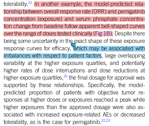
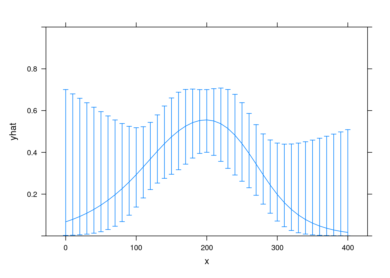
Here’s a plot exhibiting registration of my digitization of the data, using R package digitize

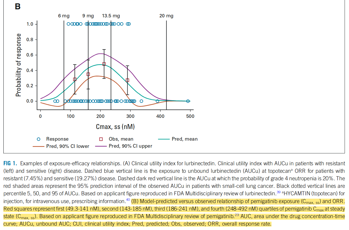
The original figure came from p 192 of this FDA CDER Multidisciplinary Review, which states, “The relationship followed a bell-shaped curve and a binary logistic regression with quadratic function was used to evaluate the relationship.”

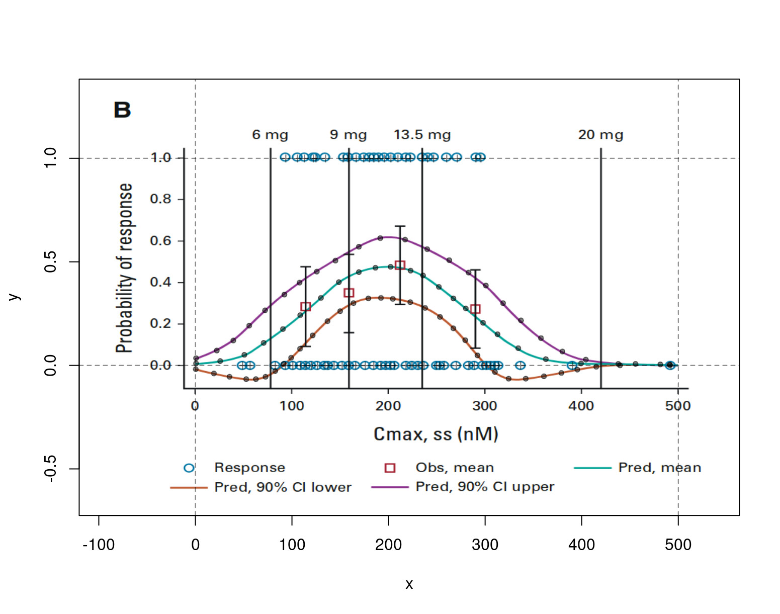
library(rms, quietly = TRUE)
fit <- lrm(y ~ poly(x,2), data = exposure_response)
xYplot(Cbind(yhat, lower, upper) ~ x
     , data = Predict(fit, x = 10*(0:40), fun = plogis, conf.int = 0.9)
     , type = 'l'
     , ylim = 0:1
       )

FYI, here is a spline regression for comparison:

fit2 <- lrm(y ~ rcs(x,4), data = exposure_response)
xYplot(Cbind(yhat, lower, upper) ~ x
     , data = Predict(fit2, x = 10*(0:40), fun = plogis, conf.int = 0.9)
     , type = 'l'
     , ylim = 0:1
       )

To evaluate the implied informational content of Figure 1B, I fitted Beta distributions to the estimated response probabilities using the method of moments — see e.g., BDA3 Eq (A.3), p583:

xout <- seq(0, 400, 25)
df <- data.frame(x = xout
               , μ = with(meancurve, spline(x, y, xout=xout)$y)
               , lcl = with(lclcurve, spline(x, y, xout=xout)$y)
               , ucl = with(uclcurve, spline(x, y, xout=xout)$y)
                 )

## Add method-of-moments estimates; see BDA3 Eq (A.3), p. 583.
df <- Hmisc::upData(df
                  , stderr = (ucl - μ)/qnorm(0.95)
                  , `α+β` = μ*(1-μ)/stderr^2 - 1
                  , α = `α+β`*μ
                  , β = `α+β` - α
                  , print = FALSE
                    )

x	μ	lcl	ucl	stderr	α+β	α	β
0	0.0088	-0.0179	0.0336	0.0151	37.4802	0.3308	37.1494
25	0.0204	-0.0451	0.0780	0.0350	15.2738	0.3115	14.9623
50	0.0493	-0.0654	0.1651	0.0704	8.4431	0.4160	8.0270
75	0.1224	-0.0500	0.2772	0.0941	11.1325	1.3630	9.7696
100	0.2099	0.0403	0.3714	0.0982	16.2103	3.4027	12.8076
125	0.3052	0.1613	0.4507	0.0885	26.0998	7.9654	18.1344
150	0.4066	0.2618	0.5199	0.0689	49.8290	20.2603	29.5687
175	0.4588	0.3196	0.5865	0.0776	40.2055	18.4459	21.7596
200	0.4761	0.3233	0.6190	0.0869	32.0648	15.2671	16.7978
225	0.4543	0.3016	0.5939	0.0848	33.4422	15.1935	18.2487
250	0.3868	0.2449	0.5391	0.0926	26.6580	10.3107	16.3473
275	0.2939	0.1437	0.4727	0.1087	16.5680	4.8694	11.6986
300	0.1974	0.0079	0.3887	0.1163	10.7113	2.1140	8.5973
325	0.1097	-0.0649	0.2703	0.0976	9.2513	1.0152	8.2361
350	0.0488	-0.0598	0.1622	0.0690	8.7612	0.4276	8.3336
375	0.0189	-0.0405	0.0789	0.0365	12.9046	0.2435	12.6611
400	0.0091	-0.0168	0.0327	0.0143	42.8959	0.3905	42.5054

To the extent that the \mathrm{Beta}(\alpha, \beta) can be interpreted as equivalent to \alpha-1 successes and \beta-1 failures in \alpha+\beta-2 Bernoulli trials (cf. BDA3 p.35), these calculations suggest that the plotted curves embody strong prior assumptions that go far beyond the data collected, and indeed beyond any data that ever could be collected, since you can’t observe fewer than 0 successes. Thus, the form of the analysis seems to have ‘put a thumb on the scale’. How reasonable does this mode of interpretation seem to the Bayesians here?

[davidcnorrismd]

Thanks to Al Maloney, who re-analyzed my own reanalysis and pointed out a likely problem with my use of poly() above, I now see I should have used rms::pol() as follows:

fit <- lrm(y ~ pol(x,2), data = exposure_response)

(As per a note in the Examples section of documentation under ?rms.trans, poly is not an rms function.)

[davidcnorrismd]

Epilogue: a PubPeer comment is now posted here:

PubPeer - Improving Dose-Optimization Processes Used in Oncology Drug...