How to interpret “confidence intervals” in observational studies

This question complements the one in the thread Random sampling versus random allocation/randomization- implications for p-value interpretation.

Given that observational studies involve neither random sampling nor random allocation, why are they riddled with “95% confidence intervals”?

7 Likes

An excellent question which I have not seen raised before. There is no frequentist interpretation if there is not envisioned population or if repeated sampling cannot be entertained. Bayesian uncertainty intervals pertain to the unknown data generating process whatever that is; it doesn’t have to involve any type of sampling. An honest Bayesian uncertainty interval would be pretty darn wide for most observational studies because you would need to have parameters describing possible effects of unknown confounders.

5 Likes

The same question could be asked for estimates of sensitivity and specificity for medical diagnostic tests, when the data used to estimate them are often generated neither from random sampling nor random allocation (ie, they used a convenience sample). Of course, as discussed on this forum previously, that may be the least of the problems with Se/Sp: Sensitivity, specificity, and ROC curves are not needed for good medical decision making

I have seen versions of this question raised before, and the heartburn comes from the obvious alternative: would I rather report point estimates without any confidence intervals at all? Sometimes I wonder if the right answer is Yes, along with showing the 2x2 table with margins. Simply report what the design of the study was, and give the results in summary tables, with no pretense of doing “statistical inference”. A descriptive summary is all the data deserves. I’ve taken this approach many times, but such tables do not allow readily exploring trends with covariates, for example. Other times I have just given the cop-out caveat, “if we were to pretend that the subjects were randomly sampled, the confidence intervals would be…”

Actually many years ago I remember Bert Gunter asking Frank about the statistical inferences in RMS Ch. 12, where the survival data for the Titanic passengers are modeled. This is a more difficult case because the model is used to explore trends in the data; it’s like an example of what Frank has said - the model may be the best way to summarize the complex structure of the data. This structure would not be evident by just making tables, I suspect. While there are no confidence intervals in the chapter, there are likelihood ratio tests; Wald statistics and p-values for different terms in the model; predicted survival probabilities for various settings of covariates, etc. Bert asked something along the lines of: to what population do these inferences apply? Sadly I do not remember Frank’s response, but the question has been stuck in my mind for 2 decades.

9 Likes

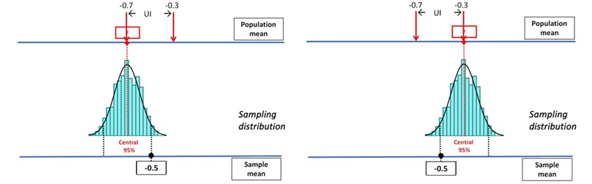
Hi Erin, random error (which UIs are about) comes from variability in the data, conditional on whatever process determined treatment and sample membership.

Systematic error (bias) is a shift between the parameter your sample truly represents and the parameter you wish it represented — and UIs don’t address that at all.

You’ve got two situations:

Sample A (nonrandom treatment allocation)

Sample not randomly selected from any defined population. Treatment is assigned by the institution’s usual, potentially biased, rules. The difference in outcomes between treatment groups within this sample is a perfectly valid random variable.

Sample B (random treatment allocation)

Same size, same male/female split. Treatments assigned randomly. The difference in outcomes now has a UI that estimates the mean difference under random assignment, which coincides with the causal contrast within this population. You can model its sampling distribution and construct a UI — for the sample’s own “internal” parameter, i.e. the true mean difference in this specific source population under those assignment rules.

In both cases, the computation of the UI is valid mathematically for the parameter tied to that specific data-generating mechanism. What changes is what parameter the UI actually refers to: In the randomised case, it can be interpreted causally (given randomisation breaks confounding). In the nonrandom allocation case, it’s about the association in that particular institutional process — not necessarily the causal effect and not necessarily the same as the population effect from the randomised study.

Why this matters for “why observational studies have UIs”

The UI itself doesn’t require random sampling or random allocation to be mathematically correct — it only needs the model for the estimator’s variability to be correct. Random sampling/allocation matter only if you want the UI to describe the same target parameter you’d care about in a broader population or under causal interpretation. Observational studies often silently assume the sample’s parameter approximates some wider target, which is where the bias vs. variance confusion creeps in.

In an observational study, you can always define a perfectly valid statistical parameter for your dataset — for example: “The mean difference in outcome between treatment and control groups in this particular set of patients under the actual allocation rules used here.” Your confidence interval is then just about random error in estimating that parameter. No problem so far. But in practice, most observational studies aren’t really interested in just this particular sample or this institution’s idiosyncratic treatment rules. Instead, they talk and think as if they’re estimating a broader target — e.g.: “The effect in the general population” or “The causal effect if treatment were assigned at random” or “What would happen if policy changed everywhere”

Authors implicitly assume that the sample parameter (what the UI is truly about) is equal to or close to the target parameter they care about. This assumption is rarely stated or justified explicitly. If it’s wrong (because of confounding, selection bias, measurement error, etc.), the UI still gives you precise numbers — but they’re precise about the wrong thing. That’s why the bias–variance confusion creeps in: Variance is what the UI reflects — uncertainty due to random error. Bias is the systematic gap between the parameter your study truly identifies and the parameter you wish you were estimating. In observational studies, bias often dominates, but the UI only talks about variance — so a “narrow” UI can give a false sense of accuracy if you silently assume the bias is zero.

In summary:
The UI in an observational study is usually fine mathematically — but if you interpret it as if it were about a different target parameter without checking the assumption that the two are equal, you’re importing bias into your conclusion without noticing. That is why observational studies take pains to eliminate bias (DAGs etc) before estimating the UI.

2 Likes

I would understand the repeated sampling to occur across multiple parallel universes of which our Universe is the sample we got. Others may be weirded out by this idea, but the notion is probably completely accessible even to the lay public through movies Sliding Doors - Wikipedia and science fiction Mirror, Mirror (Star Trek: The Original Series) - Wikipedia.

2 Likes

I don’t see that, or perhaps think it’s too much of a mind game. The beauty of Bayes is that it works equally for sample-able situations as well as one-time events. To get back to @ChristopherTong ‘s question on “what population for the Titanic” I think that the one-time event was used to illustrate methods that would be useful in more traditional situations. They don’t have a great interpretation in Titanic per se although partitioning the log-likelihood to get measures of explained variation works quite well. For confidence limits perhaps the frequentist method approximates Bayesian credible intervals that are more interpretable, as they try to uncover what we can learn about the data generating process that generated the one-time event and will never be repeated.

In the big picture, in observational data what makes confidence intervals as small as they are is assuming that uncertainties are captured. I got burned once in responding favorably to a reporter about a survey of civilian deaths in Iraq during the 2nd US Iraq invasion, because the confidence intervals were narrow enough. When Don Berry was interviewed he said that unknowns should make the confidence intervals several times wider. He was exactly correct because we later learned that the interviewers were usually too afraid to get out of their cars, and they just guestimated how many family members from that home were killed. The Johns Hopkins researchers in charge of the study never did any on-site monitoring.

In a Bayesian model if you include a bias parameter to represent unknowns, and the prior distribution for that parameter has width > 0, these uncertainties can dominate usual sampling variation-type of uncertainties. Another reason to use Bayes more often.

As another aside, frequentists frequently do sensitivity analysis for that sort of bias, simulating unmeasured confounders and determining how extreme they must be to explain away the results. The problem with that is the subjectivity in the choice of which simulation results you emphasize in the final interpretation. Bayes demands that you build the interpretation into the pre-specified analysis plan through priors. Bayes gives you a weighted sensitivity analysis to avoid biased interpretation at the end.

5 Likes

I think this old post by @Sander is worth study:

The frequentist domination of statistics has caused the emphasis on randomization as a methodology to obscure what it was supposed to do in the first place: to create exchangeable observations for comparison.

Bernardo, J. M. (1996). The concept of exchangeability and its applications. Far East Journal of Mathematical Sciences, 4, 111-122. (PDF)

This confusion stems from the language in basic stats textbooks not being formally powerful enough to represent uncertainty about the entire experimental model, which can be done using hierarchical models, as Bernardo notes in his abstract (quoted below).

The general concept of exchangeability allows the more flexible modelling of most experimental setups. The representation theorems for exchangeable sequences of random variables establish that any coherent analysis of the information thus modelled requires the specification of a joint probability distribution on all the parameters involved, hence forcing a Bayesian approach. The concept of partial exchangeability provides a further refinement, by permitting appropriate modelling of related experimental setups, leading to coherent information integration by means of so-called hierarchical models. Recent applications of hierarchical models for combining information from similar experiments in education, medicine and psychology have been produced under the name of meta-analysis.

The concept of exchangeability is fundamental to the frequentist analysis of data using permutation tests.

Good, P. I. (2002). Extensions of the concept of exchangeability and their applications. Journal of Modern Applied Statistical Methods, 1(2), 34.

I think Bernardo might be a bit extreme when he writes about coherence demanding a Bayesian approach, when he has done extensive study of reference Bayesian methods, that attempt to maximize the weight of information in the observed data, while still obtaining a proper probability distribution.

If we view any data collection effort as attempting to minimize all sources of uncertainty (ie aleatory and epistemic), we are faced with a multi-objective decision problem, which is widely known to have multiple solutions.

Related Threads

3 Likes

Uggh…thanks everyone, for trying to help me understand. Unfortunately, I too now have heartburn and will raise a glass of Gaviscon to Chris :slight_smile:

From Suhail’s post:

“Sample A (nonrandom treatment allocation)…The difference in outcomes between treatment groups within this sample is a perfectly valid random variable.”

Where exactly is the “randomness” in this scenario if the allocation isn’t random?

“Variance is what the UI reflects — uncertainty due to random error.”

I understand that a confidence/uncertainty interval is meant to reflect “random” error. But I still don’t understand what’s “random” in the observational setting…Are we supposed to treat the subjects included in observational studies like people who have been randomly sampled from the underlying population of interest? If so, then how do we justify this? When we study subjects comprising an administrative database that just happens to be available, is this process sufficiently random to allow us to say something about “random error” ? If anything, this would seem to be another example of a “convenience” sample (like we have in RCTs) (?) But in the RCT context we can at least subsequently leverage the randomness conferred by random allocation when discussing the amount of random error around the point estimate…(?)

Relatedly, in spite of everyone’s kind responses in the thread linked in the first post, I never did end up understanding how the concept of “repetition” is defined in frequentist statistics, even in the context of RCTs (which do clearly have a random component- the allocation process). Specifically, I’m still hazy on whether the hypothetical “many repetitions” of an experiment that’s imagined in the frequentist paradigm would involve the same subjects getting re-randomized many times using the same allocation procedure OR whether the imagined repetitions would involve randomization of multiple different convenience samples (with each repetition involving different subjects). In the observational setting, what exactly are we supposed to imagine that we’re “repeating” when using frequentist statistics, in order to justify generation of a “95% confidence interval”?

Question: How do we translate, in words, the following confidence interval shown in a published observational study?: “HR, 1.10 [95% CI, 1.01-1.20] )?” I understand the 1.10 part, but how can we label the interval 1.01-1.20 “random” error when there was nothing “random” in the study protocol (unless we are tacitly assuming that the subjects represented a random sample- which, arguably, is a big stretch)…

Great questions. Briefly and very coarsely my strategy is similar, e.g., to the recommendations here whereby the quality of the study design modifies my interpretation of its outputs even if they arise from the same mathematical formulas. For example, a perfectly conducted RCT gives me license to make causal descriptions, i.e., answer whether or how much treatment X changes outcome Y. For an observational study with many caveats and limitations, I use its outputs descriptively without making any causal inferences or even using it for future predictions. Instead I think: this is what these results would look like if they were a perfect RCT and use it as my yardstick for understanding the data.

Of note, while the perfect RCT would license causal descriptions, it would not in itself be able to typically answer why treatment X changes Y. For this, I would refer to mechanistic functional studies, e.g., in animal models and cell ines and in observational studies of tissue correlatives and other patient samples. The latter may also generate 95% CI that I may interpret descriptively. Thus, all datasets can be useful as long as we have the tacit knowledge to downweigh or upweigh them accordingly…

2 Likes

David Freedman once said that inferences to imaginary populations are imaginary…

My heartburn comes from the possible misinterpretation by readers seeing descriptive statistics with no confidence intervals, as that there is no uncertainty at all, especially with regard to how the results might generalize to subjects outside the sample (including future subjects). This is the motivation to at least pretend that subjects were randomly sampled or randomly allocated, to report a confidence interval, which (too-precisely) conveys a sense of uncertainty. Frank is correct that these make-believe confidence intervals likely understate the actual “uncertainty”. (And really, CIs only really convey uncertainty with respect to the presumed statistical model, and excludes model uncertainty, including the possibility of systematic error/bias, as noted by @s_doi . To borrow a phrase from Sir David Cox in another setting, the reported CIs are really just lower bounds on the actual uncertainty.) Note here that I said “motivation”, not “justification” :wink:

If anything, this would seem to be another example of a “convenience” sample (like we have in RCTs) (?) But in the RCT context we can at least subsequently leverage the randomness conferred by random allocation when discussing the amount of random error around the point estimate…(?)

My takeaway from the earlier thread is that yes, there is a bait and switch taking place when we use random sampling-based inference for RCTs based on convenience samples, when they should really be handled using random-allocation-based inference (like randomization tests and their interval estimation counterparts), but in several cases the two approaches are at least asymptotically equivalent, so that for large trials, the bait and switch results in only minor inaccuracy. For RCTs this manuever is used to make a causal link between the intervention and the outcome (internal validity), but no statistical claims of generalizability to other subjects (external validity) can be made from an RCT, except through non-statistical arguments about representativeness of the enrolled patients.

Regarding observational studies including those using administrative databases, I suspect that statistical inferences have no justification or interpretation whatsoever.

Specifically, I’m still hazy on whether the hypothetical “many repetitions” of an experiment that’s imagined in the frequentist paradigm would involve the same subjects getting re-randomized many times using the same allocation procedure OR whether the imagined repetitions would involve randomization of multiple different convenience samples (with each repetition involving different subjects).

For an RCT, in my mind it is the first - the same subjects are hypothetically re-randomized repetitively. In a designed sample survey, we would be randomly sampling different subjects from the same target population repetitively. This frequentist reasoning can feel like it’s on thin ice, and then when you have an observational study with convenience samples, I think it falls through the ice.

This does not mean I would endorse going to a non-frequentist approach. Any inference paradigm you pick cannot avoid the need for more shoe leather when working with observational data, as explained by

D. Freedman, 2008: From Association to Causation: Some Remarks on the History of Statistics, Statistical Science, 14, 243–258.

5 Likes

Thank you, Chris, this is a very clear statement.

Also very clear- thanks again.

So does this mean you have no idea what the “95% confidence interval” around HR, 1.10 [95% CI, 1.01-1.20] from an observational study actually means?

1 Like

I’m afraid so. (I’ll have another Gaviscon, please. LOL!)

Now @Pavlos_Msaouel 's comment is interesting and helpful. His interpretation might give a sense of what the lower bound of uncertainty could be, but we are still left wondering what the observational study is really telling us beyond this, and so we still need Freedman’s shoe leather. @Pavlos_Msaouel 's idea of using tacit knowledge to subjectively downweigh/upweigh the various sets of evidence is alluded to by Kay and King (Radical Uncertainty, WW Norton, 2020).

A passage in the Freedman article I cited talks about the various observational studies that collectively showed the link between smoking and lung cancer. He wrote:

Scientifically, the strength of the case against smoking rests not so much on the P-values, but more on the size of the effect, on its coherence and on extensive replication both with the original research design and with many other designs. Replication guards against chance capitalization and, at least to some extent, against confounding—if there is some variation
in study design.

This suggests that, while he thought little of “imaginary inferences”, he was not so offended as to discard them entirely, as long as they are not taken too seriously, and the factors he mentions above are understood to be more persuasive than the fake-precise p-values & CIs. Those familiar with the history of science will know that much of the knowledge-building that actually occurs follows the road Freedman describes, rather than the experimentum crucis approach that statistical inference perversely promotes. The gradual discovery of the First Law of Thermodynamics by multiple people, doing many different experiments, is an example.

Possibly also relevant is the notion of “currently subordinate factors” (of McShane et al) which should NOT be subordinate to the p-values/CIs.

https://www.tandfonline.com/doi/full/10.1080/00031305.2018.1527253#d1e248

2 Likes

Okay Erin, I will step back and start from the basics:

What is a Random Variable?

A random variable is any numerical quantity whose value could differ if you repeated the data-generating process under the same rules. It doesn’t have to come from a randomized experiment. The difference in outcomes between treatment groups in your current dataset is fixed once you have the data. But if you imagine repeating the exact same observational data-collection process, the difference would vary from run to run — and that set of possible values makes it a perfectly valid random variable. Whether it’s from a random sample or a randomized trial affects bias and interpretability, not whether it’s a random variable. You can describe it with a probability distribution.

You (and many clinicians) hear “non-random sample” and think “Oh, then statistical inference is meaningless, because it’s not random”. That’s a conceptual mistake — the mixing up two different ideas:

Random variable status – purely mathematical.

The difference in outcomes will vary from one realization of the sample to another, even if you’re pulling from a hospital database, a registry, or a convenience cohort. That variability is enough to define the difference as a random variable. You can talk about its sampling distribution, variance, and standard error. These are all mathematically sound. Your outcome difference is a random variable whether or not you had a random sample or random allocation — but without random sampling (population based data) or non-random sampling with random allocation (RCT), its interpretation changes: it reflects association in your sample’s data-generating process, not necessarily the unbiased causal effect in the target population.

Causal interpretability – a matter of study design.

If your sample was non-random (and/or your treatment assignment wasn’t randomized), the expected difference might be biased as an estimate of the causal effect. The bias comes from systematic differences between groups, not from the absence of randomness in the mathematical sense.

Practical implication in observational research

You can use statistical models to quantify uncertainty in your difference — it’s still a valid random variable. But you must be clear that your uncertainty interval is about the association in your data-generating process, not necessarily the true causal effect in the target population. This is why bias control methods (matching, weighting, regression adjustment, etc.) are so important: they aim to make that random variable’s expectation line up with the causal contrast you want.

The interval can be interpreted as the range of target hypotheses (1.01 to 1.20) whose associated data-generating models (if you repeated the data-generating process under the same rules for your data) would be judged to be a plausible explanation for the observed dataset. In this context, ‘‘plausible’’ means the observed dataset (or test statistic) falls within the central (1–α)pct of their (models 1.01 to 1.20) specified distribution of values. This definition avoids the long-run probability interpretation of the interval and shifts the focus to the realized interval.
This is why we decided to call it an uncertainty interval - uncertainty in the true data generating model given the (1–α)pct thresholds chosen for defining such uncertainty.

1 Like

If so Chris, why do Miguel Hernan and colleagues go to great lengths to emulate a target trial using observational data and then proceed to provide statistical inferences based on such designs?

I agree with that Chris, but then why are we mixing up model uncertainty with random error based statistical inference?

1 Like

There is so much great thinking here to digest. Just a few random thoughts. Sander is of course quite correct that you can make a crisp interpretation of a confidence interval, but the sure interpretation is slightly avoiding the inference question. I’m always reminded of Tukey: better an approximate answer to the right question (approximate because your prior ma disagree with mine) than an exact answer to the wrong question (how unlkely are data given an unknowable effect).

On the question of how does Bayes help protect you, think of Bayesian measurement error models that make the inference more fuzzy by the right amount, or how Bayesian joint modeling adds a parameter to allow historical data to possibly estimate something different from what is estimated in a new RCT. Adding parameters for things you don’t know makes all uncertainty intervals wider. The simplest case I can think of pertains to both observational data and RCTs: the Bayesian t-test where one quits trying to decide once and for all whether the data arise from a normal distribution and instead one adds a non-normality parameter. Again honesty in uncertainties about one parameter makes us properly more uncertain about other parameters. All while giving simple interpretations for one-time samples.

2 Likes

Thanks Suhail! I think I might be starting to see what you’re driving at (?) I’m nervous to write this, since it could be completely off-base (I’ve never thought about these issues in quite this way before), but let me know if this re-phrasing of what you’re saying resonates:

  • Frequentist statistics hinges on the idea of 1) repeating some process many, many times; 2) somehow being able to describe/model how the process actually generates its output (picturing the guts of the black box); and 3) thereby defining which outputs would be more typical versus less typical if our model is “correct”(?);
  • These repetitions don’t actually happen in real life, but rather are like thought experiments;
  • By stipulating a model (the guts of the black box), which we need to do if we ultimately want to be able to gauge the degree to which the results of our study are “typical” versus “atypical,” we are effectively defining a boundary around the universe of possible outcomes of our many repetitions;
  • In order to be able to accurately gauge which results are “typical” versus “atypical,” after defining our model for how our results will be generated, our results must at least have the potential to occupy the entire hypothetical bounded space of possible outcomes (?) As we hypothetically repeat our process and generate outcomes, over and over again, our imagined results must allow us to slowly “map” the boundaries of this universe;
  • Only if our data-generating process has some component of inherent randomness will we be able to say that, with enough repetitions, our hypothetical outcomes will slowly fill our bounded space (just as releasing smoke into a room with invisible walls will allow us to identify the boundaries of the room). And only then will we be justified in making a claim regarding the “atypicality” of any given result (?);
  • Key differences between RCTs and observational studies include 1) the nature of the repetition; and 2) where the necessary randomness comes from that allows us to define which results are typical versus atypical;
  • For RCTs, the hypothetical repetition that gets invoked is the repeated re-randomization of the same subjects to one treatment arm or another many, many times;
  • For RCTs, the randomness needed to allow us to define the boundaries of the universe of plausible outcomes is inherent in the treatment allocation process, once the convenience sample has been obtained. There is no random “sampling” from the underlying population with RCTs. Rather, we use convenience samples comprising people who are able and willing to participate- these factors hinge on many considerations including geography, whether subjects meet inclusion/exclusion criteria, and whether subjects are willing to participate;
  • For observational studies, the hypothetical repetition that gets invoked is the thought experiment involving repeated “sampling” from the underlying population of interest. If we are using an administrative database or “cohort” of subjects, we can think of them as a “snapshot in time” sample from the underlying population. The act of selecting a particular database/cohort to study is not a random process, since researchers will use databases that happen to be available to them. However, given that database membership and health status is constantly changing, there is a degree of randomness inherent in the forces that determine which members of the database would end up being considered “eligible for inclusion” in the study, from one imagined repetition of the observational study to the next (?)
2 Likes

I am afraid you are right Erin :grin:

Here is my attempt at rephrasing what you said but pardon any syntax errors as did this really quickly:

Statistical inference hinges on the idea of 1) random variation in repeated sampling from a population many, many times; 2) somehow being able to describe a probability model for the sampling variation from a population (picturing the guts of the black box); and 3) thereby defining which sample results would be more typical versus less typical if our model is “correct”(?);

These repetitions don’t need to happen in real life, if we have a probability model that we accept

By stipulating a probability model (the guts of the black box), which we need to do if we ultimately want to be able to gauge the degree to which the results of our study are “typical” versus “atypical,” we are effectively defining a boundary around the universe of possible outcomes specified under the probability model of our population;

In order to be able to accurately gauge which results are “typical” versus “atypical,” after defining our model for how our results will be generated, our results must at least have the potential to occupy the a fixed central percentage of the bounded space of possible outcomes under that model. As we hypothetically repeat our process using different population model; we generate a list of models that could have this study outcome in that central percentage of the bounded space;

The models where the data sits on the left or right side of the limits of that central percentage of bounded space are the limits of the UI.

Key similarities between RCTs and observational studies include no random sampling from the target population. Key differences between RCTs and observational studies include absence of some forms of systematic error by deign in RCTs. In both designs, randomness comes from the fact that I can have infinite sample membership possibilities;

For RCTs, the hypothetical repetition that gets invoked is the repeated sampling using the same rules for selecting participants;

For RCTs, the randomness needed to allow us to define the boundaries of the universe of plausible population models is exactly the same as with observational studies. There is of course no random “sampling” from the underlying population with RCTs. Rather, we use convenience samples comprising people who are able and willing to participate- these factors hinge on many considerations including geography, whether subjects meet inclusion/exclusion criteria, and whether subjects are willing to participate;

For observational studies, the randomness needed to allow us to define the boundaries of the universe of plausible population models is exactly the same as with RCTs. There is of course no random “sampling” from the underlying population with observational studies. The act of selecting a particular database/cohort to study is not a random process, since researchers will use databases that happen to be available to them.

1 Like

“I am afraid you are right Erin”

Hah :joy:! Totally fair. Appreciate your patience and your valiant attempt to address my misunderstandings while still retaining the skeleton of my botched phrasing. It’s not going to be a pretty sight when someone who’s never modelled anything in her life tries to understand concepts that hinge on models…

A few follow-up questions after you corrected my post (please don’t feel obliged to respond to any of them. Others reading this thread can chime in if they’re so inclined- or not, if this whole spectacle is just too sad…):

“As we hypothetically repeat our process using different population model; we generate a list of models that could have this study outcome in that central percentage of the bounded space;…”

How is the idea of different models figuring into the idea of repetition in the frequentist paradigm (?)

“The models where the data sits on the left or right side of the limits of that central percentage of bounded space are the limits of the UI.”

How do models comprise the limits of a UI, given that a UI limit is a number…?

“In both designs, randomness comes from the fact that I can have infinite sample membership possibilities;..”

Maybe I’m being overly concrete (and not thinking abstractly enough) when interpreting your wording, but how can this be true? The convenience samples we use in RCTs don’t actually have infinite membership possibilities…And, in an administrative database, it’s not true that Joe Blow from the other side of the world could ever, realistically, wind up in a UK administrative database…

“For RCTs, the hypothetical repetition that gets invoked is the repeated sampling using the same rules for selecting participants…”

Hmmm…Can I ask a very basic question? Will a statistical model that we develop/select when designing a study reflect how the people in our study happened to wind up in our study? OR does a model only represent our best guess for the shape of our outcome distribution (sorry if this phrasing is gibberish) once we’ve already defined who is going to be in our study; OR neither of the above- you can tell me to “just go read a book” if these ideas are explained somewhere in extremely simple terms…? In other words, are statistical models “blind” to the way in which our study subjects were recruited/selected for study?

“For RCTs, the randomness needed to allow us to define the boundaries of the universe of plausible population models is exactly the same as with observational studies.”

Your corrections repeatedly highlight a universe of models- a concept I haven’t yet grasped; will keep trying…

A picture is worth a thousand words - see below:

The curve with the histogram is a probability model. The population parameter is the mean of that model. The black dot is the study data. Visualize the same model but with different means moving up and down the axis. Below model -0.7 the black dot will be outside the central 95% of the histogram and above model -0.3 again the black dot will be outside the central 95% of the histogram. Hence model -0.7 to model -0.3 is the UI. We say models -0.7 and model -0.3 because all the infinite number of models are the same except for the population parameter they represent and hence models comprise the limits of the UI through their mean (population parameter). Note that the normal distribution is asymptotic so there are indeed infinite models that can generate the study data but they are beyond our rarity threshold (central 95% of the distribution specified under the model).

1 Like

One brief comment – there are definitively observational studies that inherently use sampling methods in recruitment of participants.

That’s different from whole-of-population studies including register/administrative database studies. I did some digging around recently to trace back thinking on expected variation in whole-of-population rates (e.g. cancer rates as measured from registry data for numerators and some form of population estimates for denominator) and will post that below, though that could really be its own entire thread… I would be interested if people have any citations that build on (or argue against) the arguments.

1 Like