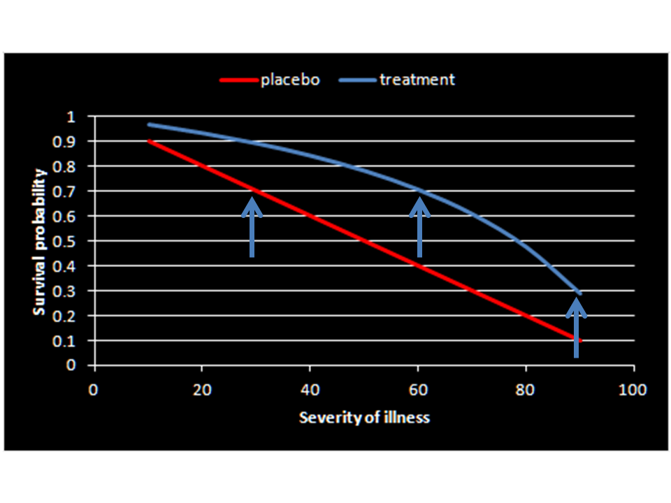
Agree Huw with your conceptualization as now its clear for a clinician to conceptualize and apply (as opposed to how it was originally described) but we now have the problem of a constant risk difference being unrealistic once baseline risks are in the impossible range. If we assume a constant fold increase in odds of survival (3.61 fold from the RCT) we get the below version of your plot. Which do you think is more realistic?
1 Like
Thanks @scott I shall check and get back to you .
As regards your solution, it seems to me that you assume, which no trialist ever does, that the control group response rate* is constant from trial to trial. I have pointed out either here or on Twitter
- That the need for concurrent control is inexplicable if one believes this.
- There are many examples where we can show this is not true (I gave two but I can easily give more).
- That representativeness is neither a feature of RCTs nor of observational studies. I gave bioequivalence studies, in which healthy volunteers are used to decide if drugs may be given to patients as an example of the former and cited a paper by Ken Rothman in support of the latter.
- That in any case it cannot reasonably be assumed that those who refuse to take a treatment would enter a trial. (I think, for example, that we can assume that those who are opposed to vaccination would not enter a trial.)
I don’t think that either you or Judea Pearl have answered these points so it would be useful to know if constancy is a necesary assumption and if so how it could be justified.
The standard statistical approach to transferring rates is to assume additivity on some useful scale (the risk difference scale is not usually a good one) so in answer tp @s_doi , Huw and I only assumed this to pick up the story as presented. Indeed something like the approach you used would be employed in practice and is discussed in my book Statistical Issues in Drug Development. See, also, for example
- Lubsen J, Tijssen JG. Large trials with simple protocols: indications and contraindications. Controlled clinical trials. 1989;10(4):151-160.
- Glasziou PP, Irwig LM. An evidence based approach to individualising treatment. British Medical Journal. 1995;311(7016):1356-9.
- I have edited my comment here to correct what I said.
2 Likes
Thanks for the interesting papers and I agree the OR scale is more realistic. Taking the latter forward, an interesting observation I have noted is that the plot using the OR as the effect measure is a ROC plot if the severity axis is replaced by Pr[Y=1| X=0,S] if we denote drug intervention as X, survival as Y and severity of illness as S. Then Pr[Y=1| X=1,S] = sensitivity (TP) and Pr[Y=1| X=0,S] = 1-specificity (FP). In this scenario, the two arms replace the expected “healthy” (placebo arm) and “diseased” (treatment arm) with the “test” being the outcome (Y). The usual diagnostic likelihood ratios can then be computed linking prior to posterior probabilities of being treated. The likelihood ratios are:
pLR = 2.333
nLR = 0.646
This means that, conditional on surviving, the posterior probability of receiving treatment for RCT members is 70%. However being negative for male gender must be associated with a nLR of 0.159 and thus for females, conditional on survival, the posterior odds of being on drug therapy is 2.333 x 0.159 = 0.37 and thus probability of 0.37/1.37 = 27%.
Now everything falls into place – patients who are destined to survive due to mild severity choose the drug therapy with Pr=0.7 but not if they are females destined to survive as then they will choose drug therapy with Pr=0.27. In either case the choice of drug therapy happens after they have mild severity and therefore will survive and therefore choosing drug has no implication for survival but is a consequence of survival. From this perspective the observational study only indicates difference in choice of male and female survivors. So seems @Scott conceptualized this the other way around when he said “…… only 27% recovery among drug-choosing women versus 70% recovery among drug-avoiding women” which perhaps should be “…… only 27% drug choice among women destined to recover versus 70% drug choice among men destined to recover”
I have written a blog Studying the Effects of Studies to explain why trialists place value on concurrent control. The TARGET study is used as an example.
1 Like
On my first exposure to the Pearl—Mueller @smueller argument (PM), my initial response was negative, because I could not (and still do not) appreciate the usefulness of involving intrinsically unobservable variables, such as pairs of potential responses, in the decision process. But, on the principle that every experience should be a learning experience, I have tried to see what of value I can extract from it. My focus may seem rather different from that of PM, but I think there are useful connexions.
There are two distinct aspects to PM that need to be kept separate:
-
The idea of combining of observational and experimental data, specifically to obtain (complete or incomplete) information about the bivariate distribution of (Y_0,Y_1) (where Y_x denotes the potential value of the response variable Y when the treatment variable X takes value x).
-
The use to be made of such distributional information (for simplicity, assumed complete) in decision analysis.
Others have commented in detail on issues related to 1. I however shall proceed on the basis that any potential problems with this have been resolved, and restrict my comments to 2, where we are concerned with the effect (for a specific individual) of a contemplated intervention, to set X=x, on the response variable Y. (Note in particular that this involves “doing”, not “seeing”, X=x).
I have found it helpful to consider a still more general case, where we have some unobserved covariate U, with
I. a known density (or probability mass function) p(u) (assumed independent of x), for U; and
II. a known conditional density p(y \mid u, x) for the observed response Y, given U and X.
There will generally also be observed covariates—e.g. patient’s sex—in the problem; we assume all distributions are assessed conditional on the patient’s values for these, so we initially omit them from the discussion.
Note that the above conditions hold, formally at least, in the PM context, on taking U = (Y_0, Y_1). Then I is obtainable (at least in the simple case we consider here) from the combination of observational and experimental data; while II holds with the deterministic relation Y = Y_X, so that {\rm P}(Y = y_x \mid (y_0, y_1), x) = 1.
The decision tree grows as follows. First, a value x for X is chosen. Next, Nature generates the pair (Y,U) (the order being immaterial), with joint density p(u) p(y \mid u, x). Finally, a loss L(x,y,u) is suffered. The optimal choice of x minimises {\rm E}\{L(x,Y,U) \mid X=x\}, the expectation being computed with respect to the above density p(u) p(y \mid u, x) of (Y,U) given X=x.
Now {\rm E}\{L(x,Y,U) \mid X=x \} = {\rm E}\{L^*(x,Y) \mid X=x \}, with
L^*(x, y) = {\rm E}\{L(x,y,U) \mid Y=y, X=x\},
involving the conditional distribution of U given (x,y), which has density
p(u \mid x, y) = p(u) p(y \mid u, x)/\int p(v) p(y \mid v, x) dv\qquad(*)
This will typically depend on both x and y.
So the optimal x will minimise {\rm E}\{L^*(x,Y) \mid X=x\}, using the distribution of Y when X=x.
Now in a clinical trial setting one would normally ignore unknown covariates, assign terminal loss L(y) depending only on the eventual response y, and aim to minimise {\rm E}\{L(Y) \mid X=x\}. Equivalently, for binary Y, one would aim to minimise {\rm P}(Y=1 \mid x), the probability of the (undesirable) outcome 1, consequent on choosing action x. This would accord with the above more detailed decision analysis above so long as L^*(x,y) is a function of y alone.
When will this be the case? It will hold if our terminal loss L(x,y,u) is of the form L(y) – ignoring U and also X – in which case also L^*(x,y) = L(y), and we recover the usual analysis.
What if the terminal loss is L(y,u), depending on the patient’s unobserved characteristics U as well as on the response Y (but not on the treatment x applied)? This seems to me a perfectly reasonable assumption. Then L^*(x,y) = {\rm E}\{L(y, U) \mid X=x, Y=y\}, the expectation being with respect to (*), and this will typically involve x – in which case the analysis will differ from the usual one. In such a case @Stephen’s dictum “We have no choice but to play the averages” would be inappropriate.
An exception to this dependence on x will be when U is independent of X, given Y. Since U is in any case independent of X, this will hold if either
a) Y is independent of U, given X – in which case U has no predictive value; or
b) Y is independent of X, given U – in which case Y and U are jointly independent of X, so that treatment makes no difference to anything, and we can do whatever we want.
By a result of Yule, the above sufficient condition “(a) or (b)” is also necessary when Y is binary. Then, unless (a) or (b) holds, it will be crucial to take account of the dependence of the loss on the unmeasured individual characteristic U.
Consider the following toy example. Take all variables binary; U = 0 or 1, each with probability 0.5; and Y = 0 if U=X, else 1. That is, the patient will recover if and only if the treatment applied happens to agree with the patient’s unobserved characteristic U. In particular, under either treatment, the marginal probability of recovery is 0.5, so if this is all we care about it won’t matter what we do.
Now suppose the loss is L(y,u) = y+u, with two components: the first is 0 if the patient recovers, else 1; the second is the value of U: patients with U=1 have a worse quality of life. Then L^*(x,y) = y + {\rm E}(U \mid X=x, Y=y), and I compute
L^*(0,0) = 0
L^*(0,1) = 1
L^*(1,0) = 2
L^*(1,1) = 1.
So L^*(x,y) depends on x as well as on y.
Finally, the expected loss for X=0 is 0.5, whereas that for X=1 is 1.5. So, under this elaboration of the problem to incorporate dependence of the loss on U, we get a different solution, with X=0 the optimal act.
Consider now the sort of problem addressed by PM: to decide which patient or patients to treat. Different patients will have different observed characteristics, which will affect the individual probabilities to be used in the above analysis. For our toy example, the overall value of treating this particular patient was 0.5. We might do a similar analysis for other patients, and compute the aggregate value of treating some specified subset, finally choosing the optimal subset (perhaps under resource constraints). The individual decision problem considered above remains however a basic building block for such an extended analysis.
How does all this work in the specific PM set-up, with U = (Y_0, Y_1)? As I understand it, the idea is that, if we treat a patient who then recovers, it is considered better if that patient would not have recovered if left untreated, than if the patient would have recovered anyway. We might thus take, e.g., L(x, y, (y_0, y_1)) = 0 if x=1, y=1 and (y_0, y_1) = (0,1), 1 otherwise. (The paper Unit Selection Based on Counterfactual Logic, by Ang Li and Judea Pearl, Unit Selection Based on Counterfactual Logic | IJCAI, allots different utilities to the 4 possible configurations of (y_0, y_1), though it is not clear to me how these might vary further with x and y). Any way, given some such assessment of loss or benefit, we can formally proceed with the general argument outlined above.
I still do not like PM’s focus on the “covariate” U = (Y_0, Y_1), which is not only unobserved but unobservable. For my generalization above, I would want the covariate U to be a real, potentially observable, quantity, even though not observed in the problem at hand; together with a carefully considered loss function L(y,u) (only rarely would I expect dependence on x to be appropriate).
In spite of these differences, there is a common moral to both the PM approach and my own: when we consider that the (negative) value of an outcome could depend also on the value of some personal information, even when that information is not available, we should take that into account in setting up an appropriate loss function for the decision problem, and not, as is usual, ignore this extra information. It is in that sense we need to do personalised medicine.
3 Likes
… go get it anyway! [1]
- Jones, M. R., K. A. Schrader, Y. Shen, E. Pleasance, C. Ch’ng, N. Dar, S. Yip, et al. “Response to Angiotensin Blockade with Irbesartan in a Patient with Metastatic Colorectal Cancer.” Annals of Oncology: Official Journal of the European Society for Medical Oncology 27, no. 5 (2016): 801–6. Open access
Happy New Year everybody!
1 Like
If you can observe it, fine – it then becomes part of the background information that, by assumption, has been conditioned on. At which point we can start the process again, with that now behind us, and with a new unobserved covariate U.
But note that, in the context of the original PM proposal, with U = (Y_0,Y_1), it is logically impossible to observe U.
1 Like
It seems safe to say that a formulation of individual response unable to account for the individual’s response in Jones et al (2016) has no merit.
I can’t disagree with that.
1 Like
In response to @PhilDawid‘s “aspect 1: “The idea of combining of observational and experimental data …”, my understanding is that P&M’s aim was to establish a principle that data from RCTs can be supplemented by an observational study to reveal hidden facts not already addressed in a RCT that can improve clinical decision making. This aim is set out in @Scott’s preamble in post 8. However, although I provided an explanation for their data in post 5 above, it was not the one P&M had intended.
I have restated the problem using different simulated data based on collapsible odds ratios (instead of their example based on collapsible risk differences), which is a more familiar situation for a physician like me (and perhaps statisticians like @stephen and @f2harrell). The result of such a RCT might look like this:
| Table 1: All subjects | Placebo | Treatment | Totals↓ |
|---|---|---|---|
| Alive at time T | 1160 | 1580 | 2740 |
| Dead at time T | 840 | 420 | 1260 |
| Totals→ | 2000 | 2000 | 4000 |
The odds ratio as a measure of treatment effect here is (42/158)/(420/1580) = 0.37. The probability of being dead at time T on placebo is 0.42 but on treatment it is 0.21.
P&M wondered whether the result of a RCT like that above could contain hidden differences and I agree. If we divided the subjects into those with mild and severe illness (instead of male and female), then the results for those with a mild illness might look like this:
| Table 2: Mild illness | Placebo | Treatment | Totals↓ |
|---|---|---|---|
| Alive at time T | 960 | 1308 | 2268 |
| Dead at time T | 40 | 20 | 60 |
| Totals→ | 1000 | 1328 | 2328 |
The odds ratio here is again (20/1308)/(40/960) = 0.37. However on this occasion the probability of death on placebo is only 0.04 and on treatment it is 0.015, an absolute risk reduction of only 0.025.
If we consider those subjects with severe illness the result might look like this:
| Table 3: Severe illness | Placebo | Treatment | Totals↓ |
|---|---|---|---|
| Alive at time T | 200 | 272 | 472 |
| Dead at time T | 800 | 400 | 1200 |
| Totals→ | 1000 | 672 | 1672 |
The odds ratio here is again (400/272)/(800/200) = 0.37. However on this occasion the probability of death on placebo is 0.8 but on treatment the probability is 0.6, an absolute risk reduction of 0.2.
These examples confirm P&M’s suggestion that trials can hide important information unless a predictive piece of conditional evidence is also incorporated into the trial (e.g. the albumin excretion rate in a RCT to assess the effect of irbesartan on the outcome of nephropathy [1]). From a medical point of view, the result of the above RCT might give rise to a clinical guideline that in view of the side effects of treatment, subjects with mild illnesses should not be treated as any improvement in prognosis of 2.5% would be outweighed by the risk of other adverse outcomes. However, severe patients would gain an increased prognosis of 20% and should be treated.
An observation study based on an audit of this guideline during day to day care should then demonstrate 4% mortality at time T on those not treated but 60% mortality in those treated. Such an outcome of an audit of the guideline would be as expected and acceptable. The counterfactual results of 80% mortality in severe patients on placebo and 1.5% mortality for mild patients on treatment would not be available from observations of applying a guideline of course. If the results were very different to the above then it would call into question the effectiveness of the guideline or the efficacy suggested by the RCT.
Perhaps such a follow-up study could also be used to estimate a risk ratio based on the conditions of exclusivity, relevance and randomness used by Angris, Imbens and Rubin. If an original RCT had not explored the role of disease severity then it could be done during such an observational study by using a suitable test that represented disease severity (e.g. the albumin excretion rate [1, 2]. Observational studies could also be used to compare the predictive properties of a variety of such tests. I suggest such an approach in Section 3.4 of the following pre-print: https://arxiv.org/abs/1808.09169 [2], the bulk of the paper being about a similar approach based on randomising to different diagnostic strategies instead of directly to intervention and control. Judea P criticised a previous version for not discussing issues of causal inference amongst other things, which I have now addressed in detail in section 5.1 to 5.7.
All this is from the viewpoint of an experienced physician and clinical teacher with no formal training in mathematics but a wish to understand his own diagnostic and decision making processes with mathematical clarity. I would be grateful for any comments and advice about this post, including about the pre-print in Reference 2 if possible.
References
-
Llewelyn H. The scope and conventions of evidence-based medicine need to be widened to deal with “too much medicine”. J Eval Clin Pract 2018, 24, 5, 1026-1032. https://onlinelibrary.wiley.com/doi/10.1111/jep.12981
-
Llewelyn H. Preprint in arXiv: [1808.09169] The probabilities of an outcome on intervention and control can be estimated by randomizing subjects to different testing strategies, required for assessing diagnostic tests, test trace and isolation and for natural randomisation
Beautiful. I want to offer a big-picture perspective at this point. When the RCT has a reasonable spectrum of patient types, it is not so clear what the observational data brings to the table other than providing a broader basis for estimating absolute outcome risks under standard treatment. Taken with the estimate of relative efficacy (e.g., odds ratio) from the RCT one can then get better estimates of absolute risk under standard and new therapies. The main drawback of using just the RCT would occur if the investigators were not bright enough to explore the impact of baseline disease severity while analyzing the trial results.
5 Likes
I want to make sure I am getting it right. Do you mean calculating the risk difference distribution? like you have done here:
Yes but this is a slightly more relevant article: EHRs and RCTs: Outcome Prediction vs. Optimal Treatment Selection | Statistical Thinking
1 Like
Practically it is often challenging to rely only on RCT data when making inferences about patients we see in clinic. This is because RCTs, being experiments, prioritize patient selection over representativeness to reduce variance and maximize the information gained on relative treatment efficacy. These inferences need to be fused with large-scale observational data to facilitate patient-specific inferences.
Thus, I think Pearl and @scott have their hearts in the right place even if I do certainly share the concerns stated in this thread and on twitter. Here is a more mature attempt for such fusion between RCT and observational datasets.
1 Like
I join Stephen in his amazement.
Granted, there are ill-defined RCTs and there can be biased/confounded observation. The case presented in the blog displays a surprisingly large gap between RCT and observation data yet claiming that both are based on similar population. Neither can RCT answer counterfactual questions down to individual cases, nor can observational data as long as only statistical information is available. Pearl’s rung 3 requires deterministic modeling / knowledge.
Observational data may help refine RCT, assessing confounding factors and thus e.g. trying to zoom in as much as possible towards a sub-population of interest. But if observation contradicts well-defined RCT results then it probably misses a lot of important features or is plagued by selection biases. RCT is also useful to find or prove causal arrow direction.
Data proposed in the blog can be modeled with following causal Bayesian network.
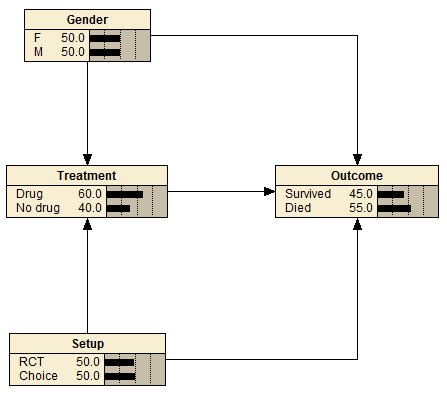
Treatment:
Drug        No drug     Gender Setup
0.5         0.5         F      RCT
0.6998      0.3002      F      Choice
0.5         0.5         M      RCT
0.6998      0.3002      M      Choice


Gender:
F           M
0.5         0.5


Outcome:
Survived    Died        Treatment Gender Setup
0.489022    0.510978    Drug      F      RCT
0.270328    0.729672    Drug      F      Choice
0.49002     0.50998     Drug      M      RCT
0.699715    0.300285    Drug      M      Choice
0.210579    0.789421    No drug   F      RCT
0.699336    0.300665    No drug   F      Choice
0.210579    0.789421    No drug   M      RCT
0.699336    0.300665    No drug   M      Choice


Setup:
RCT         Choice
0.5         0.5
1 Like
As @stephen and others have written before, RCTs do not require representativeness in the usual sense, and do not profit from it aside from specific issues surrounding interactions.
1 Like
Which is exactly why RCTs alone usually cannot be used for patient-specific inferences, i.e., at rung 3 of Pearl’s ladder of causation. For that we need additional knowledge and assumptions.
The same applies for all well-designed experiments, including those we do in the lab. Alone they are not enough to guide any major decisions. Knowledge from multiple domains needs to be integrated.
1 Like
I totally accept the principle as pointed out by you @f2harrell and @stephen that RCTs can only be expected to estimate risk ratios or odds ratios from ‘non-representative’ populations and that this information is applied to an individual by using her or his personal baseline risk of the trial outcome. However this baseline risk should not be estimated in any old way. (For example some cardiovascular risk calculators will predict that a lipid lowering drug will reduce CV risk in a person with an extremely high blood pressure when the lipid levels in that person are impeccably low risk!)
The baseline risk should be based on a data examined during the trial (e.g. as disease severity or staging) by the investigators in planned way. If this was not done at the time (as by @Scott and JP), I can’t see a subsequent ad hoc observational study as suggested by @Pavlos_Msaouel, @Scott and JP providing the required baseline risks. It will need another RCT or planned study by randomising to different test thresholds (or different tests) as described in my recent pre-print [1] and the chosen model based on collapsible ORs or RRs calibrated as described in Section 5.7 and Figure 5 of that pre-print. The principle behind this design is to assess the RR or OR in a sub-population where there is equipoise. The population is therefore highly non-representative. Section 2.1 of the preprint sets out the assumptions on which this is based (the subsequent proof for this is in section 5.1 and thus why ‘representativeness’ is not required in general).
@Stephen has been very supportive of my ideas. Do you or anyone know of other groups who are trying to do something similar to me?
Reference
1 Like
Why not? When making individualized inferences we have to assume that the patient we see in clinic shares certain stable causal properties with the RCT population. One could indeed assume that this causal structure is only present in the RCT cohort and apply the RCT findings only to patients from the exact same population, including the center they were treated and all other eligibility criteria. But no clinician ever does that, certainly not in oncology. Instead, we assume that the patient we see in clinic shares the same key causal structures that allow the transportability of inferences from an RCT that may, for example, have been done in a different country. This is a reasonable approach, in part because the RCT eligibility criteria are often very poor discriminators of patient baseline risk, as opposed to large-scale observational studies to develop prognostic risk scores.
But now note that the assumptions needed to transport RCT inferences to the patient we see in clinic are generally stronger than the ones needed to integrate knowledge on the relative treatment effect from RCTs with knowledge on baseline risks from observational datasets.
I am writing a paper on this with the hope that it will be accessible to statisticians and methodology-minded clinicians. The biggest challenge is notation. Each community focuses on different aspects of a problem and uses their own terminology and mathematical notation, and this can be confusing. I was raised within the Bayesian statistical school and I am much more familiar with that notation. But for this and other related projects, in the past few months I dived much more into the notation used by computer scientists to also help our statistical collaborators digest and incorporate it in our work. It is not an easy task but it is well worth it.
As a very simple but practical example of how valuable this integration can be, see this post discussing how problematic it can be to judge a surrogate endpoint based on how strongly it correlates with overall survival. Instead, we need first to consider the causal networks that generated these endpoints.
3 Likes
I challenge that statement. If the RCT’s patient entry criteria are reasonably broad, the RCT provides the best data for estimating outcome tendencies of the patients in the control arm. Among other things, RCTs have a well-defined time zero and do not lose patients to follow-up. Observational data, besides having higher measurement error and often tragically higher amounts of missing data, tend to have trouble deciding exactly which patients to include in the analysis and trouble keeping track of patients in follow-up.
2 Likes