Individual response

[Raj]

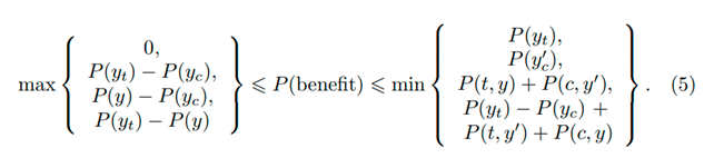
Huw has asked me to add a few additional thoughts on the topic of “how to best calibrate outcome probabilities”

From what I can gather in the previous comments, the majority of this discussion has been on improving calibration of various models for medical outcomes, which remains a very important topic.

However, in my experience most physicians rely on their own “internal thought process” to estimate (or gestalt) outcome probabilities, which are then used for decision making. But physicians are not always good at these sort of estimates. Our clinical experience helps us refine our ability discriminate between various predictors/risk factors to determine the most likely outcomes, but it does not (on a case by case basis) always calibrate those same estimates.

Thus, the “best” way improve this process would require calibrating physicians estimations. Ideally, models are best suited to provide some external validity or check against which we as physicians can see if our internal estimates match external ones. At the moment, our best bet is to have peer to peer discussions, and thus calibrate our judgement to a consensus. This is, however, not ideal.

A large part of physician education focuses on improving our diagnostic skills. No one wants to make a mistake. So we focus on the various ways we might error. A lot of this involves cognitive psychology and various forms of cognitive biases.

But it is equally important that our predicted outcomes have some external measure, so that from time to time physicians can also calibrate their estimates against validated models, and not just the opinion of our peers.

In order for this process to be acceptable, its is important that those external models be transparent, and the assumptions clearly understood. We need to ensure the physicians can have confidence against which we calibrate our internal thought process, or the limitations of any model should we have disagreement.

[f2harrell]

These good thoughts remind me that there is a vast literature on this subject in psychology, led by visionaries such as Robyn Dawes. Psychology experiments have shed a light of light on many aspects of the problem, including how misunderstanding probabilities subverts decision making, and how practitioners can learn to update their probabilities to make them better calibrated. Another aspect is the “lens model” whereby one analyzes cues on which a decision is based in order to understand which cues are emphasized. In some examples it was found that the “expert” decision makers were giving weight to less important cues and no weight to dominating diagnostic or prognostic variables.

[llynn]

This is a great discussion. My teams work on ML and AI led me to be very concerned about the need for bedside computational transparency to allow continued calibration by physicians in the presence of AI. Existing protocols are calibrated routinely by physicians, black box decisions would remover physician calibration in exchage for the AIs processing. The alternative is computationally transparent AI.

This is the present state with physician//nurse calibration:

This is the black box state:

Artificial intelligence systems for complex decision-making in acute care...

[scott]

@HuwLlewelyn I apologize for the late response, I’ve recently become aware of new activity on this thread and noticed I hadn’t responded to a previous post of yours.

@HuwLlewelyn

My understanding from this is that p(yt|t,male) [or alternatively p(yt|t,female)] is based on a 3rd scenario, where the male subject chooses treatment or no treatment and is then supervised with care as in a RCT.

P(y_t|t, \text{male}) is the same thing as P(y|t, \text{male}) due to consistency. So this isn’t a 3rd scenario, it’s the same thing as your 2nd scenario.

@HuwLlewelyn

For males p(y’t|t,M) = 0.3 and p(y’c|c,M) = 0.79 so that p(Benefit|M) = 0.79-0.3 = 0.49.

P(y'_c|c,\text{male}) = P(y'|c, \text{male}) = 0.3. I’m not sure how you got P(y'_c|c,\text{male}) = 0.79 or why P(\text{benefit}|\text{male}) would be equivalent to P(y'_c|c,\text{male}) - P(y'_t|t,\text{male}).

@HuwLlewelyn

I still can’t identify the assumptions that you have made and therefore don’t understand why p(Harm) = p(Benefit) – ATE

Not many assumptions were made, just the basics. Consistency, no selection bias in the RCT and observational studies, no measurement error, etc. Here’s a proof of the relationship between harm, benefit, and ATE, considering that P(\text{benefit}) = P(y_t, y'_c) and P(\text{harm}) = P(y'_t, y_c):
\begin{aligned}\text{ATE} &= P(y_t) - P(y_c)\\&=[P(y_t, y_c) + P(y_t, y'_c)] - [P(y_t, y_c) + P(y'_t, y_c)]&&\text{law of total probability}\\&= P(y_t, y'_c) - P(y'_t, y_c)\\&=P(\text{benefit}) - P(\text{harm}).\end{aligned}

@HuwLlewelyn

It may be that your definitions of benefit and harm are different to mine and statisticians such as @f2harrell and @stephen

What is your definition of benefit of harm? My definition is expressed best in the probabilities mentioned above: P(\text{benefit}) = P(y_t, y'_c) and P(\text{harm}) = P(y'_t, y_c). In words, the probability of benefit is the probability of positive outcome if treated and negative outcome if untreated. The probability of harm is the probability of negative outcome if treated and positive outcome if untreated.

@HuwLlewelyn

According to this definition, harm and benefit cannot happen at the same time in a RCT result that focuses on one outcome.

Imagine the individuals in an RCT. If 40% of the treated are cured and 40% of the control are cured, then the ATE is 0. That doesn’t mean none of the individuals benefited from treatment, nor does it mean that none of the individuals were harmed by treatment. It could be, in the extreme case, that all 40% of the treated benefited from the treatment. They were cured because of the treatment and would not be cured had they not be treated. At the same time, another 40% of the population are harmed by treatment. They weren’t cured because of being treatment and would’ve been cured had they not been treated. That’s why you see 40% of the control group as having been cured. The average effect is 0, but individually 40% benefit and another 40% are harmed. We would then say P(\text{benefit}) = P(\text{harm}) = 0.4 and \text{ATE} = 0. Does this help spell out my definition of benefit and harm?

@HuwLlewelyn

Would it be possible for you to apply your approach to risk ratios instead of risk differences in order that a better comparison can be made with a physician’s approach to personalised risk assessment?

Yes, this might be interesting, I’ll play with this.

In Section 3 of our paper, we wrote, “although men and women are totally indistinguishable in the RCT study, adding observational data proves men to react markedly different than women, calling for two different treatment policies in the two groups. Whereas a woman has a 28% chance of benefiting from the drug and no danger at all of being harmed by it, a man has a 49% chance of benefiting from it and as much as a 21% chance of dying because of it.”

I’m curious, does this make sense? If not, which part is problematic?

[scott]

@Pavlos_Msaouel

Take a look if you get a chance as I am looking forward to seeing whether the way we approach these patient scenarios can be integrated with the concepts you are developing.

I just printed your paper and am excited to read it.

[HuwLlewelyn]

Thank you @Raj. An anecdote … I once had a trainee doctor who was excellent (and subsequently became a professor of medicine). However when he was with me he kept failing his post grad exams because he was hopeless at multiple choice questions. When I looked into this he did not seem to distinguish well between probabilities of being right. I got him to keep a notebook of his personally estimated probabilities of the results of tests requested by him that would subsequently fall within a specified range. For each of his estimated probabilities, he then counted how often he was right. Very soon he became well calibrated. He then passed his exams. Maybe all medical students and doctors should do this privately to hone their clinical judgements. However we need very general and widely acceptable ways of calibrating such probabilities especially when data is sparse. Maybe @f2harrell could lead the charge!

[ESMD]

Primary care is a rapidly-humbling endeavour in this regard.

A simple, common clinical example: every week, primary care physicians see patients who report that they are losing hair. Patients wonder what the cause might be. They have usually “googled” the problem before the appointment. “Do you think I’m deficient in some type of vitamin?” “Do you think it could be my thyroid?”…

All MDs learn in medical school that hypothyroidism can cause hair loss. So pretty much every patient who reports hair loss gets his/her sTSH level checked. But after checking the sTSH in thousands of patients reporting hair loss, over many years of practice, it dawns on MDs that the test only comes back abnormal in a miniscule proportion of cases. And in fact, all the other lab tests for hair loss usually also come back negative. So the PCP, over time, learns to temper patients’ expectations, right from the initial visit. We caution that there is unlikely to be an easily treatable underlying cause or an easy solution for the problem.

It’s curious how, in spite of reading that a high proportion of many medical conditions are “idiopathic,” MDs don’t seem to really internalize the meaning of this word until they have been practising for many years. Some type of clinical prediction tool that could be used, early in training, to speed up this internal calibration process could be very useful in helping to manage patient/MD expectations. But at the end of the day, we will still probably end up checking the sTSH (because nobody would want to miss an “easy-fix”)…

[HuwLlewelyn]

Thank you @Scott. I shall try to identify the difference between the way you and I view the concept of harm and benefit. If the probability of a desired outcome on treatment exceeds the probability of that desired outcome on control then this difference in probabilities is regarded as a ‘benefit’. This is of course known as the average treatment effect’ (ATE, e.g.of +0.2). The latter is not a probability but the difference between two probabilities. ‘Harm’ is when the probability of a desired outcome on treatment is lower than on control, when the ATE is in the opposite direction (e.g. -0.2). Clearly the ATE cannot be positive and negative at the same time. A treatment effect can also be measured as the difference between two means in terms of the number standard deviations or standard errors of the mean.

If the above are assumed to be ‘true’ probabilities based on an infinite number of observations, a real study would be based on a limited number of observations that might provide a P value based on a null hypothesis of no difference between the probability of an outcome on treatment and control. By assuming uniform prior probabilities we could say that the probability of a ‘true’ positive ATE conditional on the data in favour of treatment greater than zero would be 1-P. This would be a probability of benefit. A probability of a negative ATE conditional on data would be that of harm.

By contrast, it appears that your concept of a benefit and harm is a pair of observations (e.g. a combination of an observed desired outcome on treatment and a counterfactual observed desired outcome on control). The control outcome can be envisaged as going back in time to before a treatment had been given and then administrating the control action and then observing the outcome. This can result in 4 possible scenarios: 1-A desired outcome on treatment and control, 2- A desired outcome on treatment but not on control (i.e. ‘benefit’), 3-An undesirable outcome on treatment but a desired one on control (i.e. ‘harm’) and 4- An undesired outcome on treatment and control. The proportion of times each of these scenarios occur gives rise to the probabilities of them occurring. Therefore if scenario 2 occurs occurs 30% of the time in some population then the probability of benefit is 0.3. Therefore if scenario 3 occurs occurs 10% of the time then the probability of harm is 0.1. I will now consider an example with your notation.

1. If an individual has a good outcome Y on a treatment T and then in a counterfactual situation (e.g. by going back in time to before the treatment was given) there is also a good outcome Y on control C, then that is an INDIVIDUAL ‘NO CHANGE’ from treatment (represented by Yt, Yc as in ‘1-Same outcome’ in Tables A and B)
2. If an individual has a good outcome Y on a treatment T and then in a counterfactual situation (e.g. by going back in time to before the treatment was given) there is not a good outcome Y’ on control C, then that is an INDIVIDUAL BENEFIT from treatment (represented by Yt, Y’c as in ‘2-Individual benefit’ in Tables A and B)
3. If an individual does not have a good outcome Y’ on a treatment T and then in a counterfactual situation (e.g. by going back in time to before the treatment was given) and there a good outcome Y on control C, then that is an INDIVIDUAL HARM from treatment (represented by Y’t, Yc as in ‘3-Individual harm’ in Tables A and B)
4. If an individual does not have a good outcome Y’ on a treatment T and then in a counterfactual situation (e.g. by going back in time to before the treatment was given) there is not a good outcome Y’ on control C also, then that is an INDIVIDUAL ‘NO CHANGE’ from treatment (represented by Y’t, Y’c as in ‘4-Same outcome’ in Tables A and B)

In Table A, the pair of columns on the right show that more have a good outcome on treatment than control in a RCT (i.e. 0.5 or 50% compared to 0.3 or 30%) so treatment shows benefit with an ATE of 50-30 = plus 20%. In Table B, more have a good outcome on control than treatment, so treatment shows harm with an ATE of 30-50 = minus 20%.

However, for the RCT result in Table A and for the Observational Study result in Table B, there are unlimited possible scenarios of individual benefit and harm as illustrated by three individual scenarios. Note that p(Benefit)-p(Harm) for the 3 different counterfactual scenarios in Table A are 0.2-0 = 0.3-0.1 = 0.4-0.2 = +0.2 ATE. There are an unlimited number of such possibilities that all map to an ATE of +0.2. In Table 3 we get 0-0.2 = 0.1-0.3 = 0.2-0.4 = -0.2 ATE, with also unlimited possibilities that map to an ATE of -0.2. HOWEVER, the opposite is not true in that an ATE of +0.2 or -0.2 does not map to an unique combination of p(Benefit) and p(Harm) but to an unlimited number of possible combinations.

If the right hand side of Table A was the result of a RCT and Table B was the result of an observational study you claim that you can determine which patients and in what proportion experienced individual benefit and individual harm and no change. It seems to me that you estimate various upper and lower bounds of the values in these ‘individual scenarios’ based on a number of assumptions and in your paper find that the latter are equal, thus allowing you to get point estimates. However, it is not clear to me what the assumptions are especially when applied to particular situations like an RCT and an observational study. However, if for example the RCT’s ATE is positive and the Observational Study’s ATE is negative, there can be no common set of values in their respective scenarios as all the p(Benefit) - p(Harm) = ATE in one group are positive and all the p(Benefit) - p(Harm) = ATE in the other group are negative. For example, if x = p(Benefit) and y = p(Harm), ATE from RCT = a and ATE Obs Study = b, can these be used to form a pair of soluble simultaneous equations? Can you suggest a scenario that provides a p(Benefit) and a p(Harm) that is common to both groups?

[davidcnorrismd]

@Pavlos_Msaouel

models informed by mechanistic knowledge

I’m struck by how much of the work of transportability your “mouse-to-man assumption” and other “key assumptions” are doing in this paper. I’m left wondering what precisely the DAGs contribute to the undertaking!

If anything, the DAGs might be obscuring the fundamental importance of preclinical work. Statements such as:

Using this diagram, we can determine whether we possess sufficient knowledge to make such cross-population predictions for patients seen in clinical practice.

actively mislead as to the necessary-but-not-sufficient character of causal graphs as (merely) a formal logic of identifiability.

[Pavlos_Msaouel]

@davidcnorrismd

If anything, the DAGs might be obscuring the fundamental importance of preclinical work.

Not sure I follow. We effectively use DAGs in preclinical research all the time. As an example, take figure 2 here whereby three different DAGs are used to represent the putative mechanisms that could have generated the observed survival distribution. Only one of these DAGs would indicate that targeting the HIF pathway would be helpful to patients. We thus design preclinical and clinical experiments for causal discovery that can refute each of the three DAGs.

[davidcnorrismd]

I should perhaps have clarified that I meant DAGs were obscuring the matter specifically in your paper. Notably, Kaelin’s Figure 2 employs simple DAGs in a critical mode to exhibit necessary considerations to avoid a pitfall. Your language as quoted above, by contrast, falsely implies sufficiency.

[Pavlos_Msaouel]

I see. Good point. That quote would indeed have been more accurately stated as “Using this diagram, we can determine whether we possess necessary knowledge to make such cross-population predictions for patients seen in clinical practice”

[scott]

@HuwLlewelyn

The control outcome can be envisaged as going back in time to before a treatment had been given and then administrating the control action and then observing the outcome.

Yes, this is the concept I refer to when I mention benefit. The difference between basing benefit on ATE vs P(y_t, y'_c) is the former is average benefit and the latter is individual benefit. To me benefit should always be (y_t, y'_c) because the word connotes whether a treatment helped you. Even if \text{ATE}=0, the treatment could’ve helped/benefitted some people.

Your Table B has observational results but experimental notation. Is Yt supposed to be P(y|t) or is it an observational study with results adjusted to provide the causal effects, such as P(y_t)?

If you want to play with RCT and observational data to see the effect on benefit and harm, we made this little interactive plot: https://lbmaps.web.app/

[HuwLlewelyn]

Thank you @scott. I have amended the notation in Tables A and B to make it more explicit (I’m sorry that I had taken a short-cut with my initial version, hoping that you would understand what I was getting at). According to my understanding of Tables A and B it would not be possible to identify a counterfactual scenario that satisfied the result of a RCT where the ATE was positive (as illustrated by the 3 counterfactual scenarios in Table A) and an Observational Study where all the ATE was negative (as illustrated by the 3 counterfactual scenarios in Table B). If the ATE was zero, there could also be an unlimited number of possible counterfactual scenarios where there are different values of p(Benefit) = p(Harm). I suppose it all hinges on the assumptions that you make in your paper to insert the probabilities in equation (5) below to give upper and lower bounds of p(Benefit), which i confess that I find difficult to follow . Another problem is of course that it does not seem possible to confirm the truth of these assumptions, at least by going back in time and actually seeing what would have happened if things had been done differently (with the exception of course that we can safely assume that 0≤ p(Benefit) ≤1, for example!). Do you have some other ways of verifying your assumptions?

[scott]

@HuwLlewelyn

If the ATE was zero, there could also be an unlimited number of possible counterfactual scenarios where there are different values of p(Benefit) = p(Harm)

Yes, if P(\text{benefit}) is a range, then it can be any real number within that range. Since \text{ATE}=0, P(\text{benefit})=P(\text{harm}).

@HuwLlewelyn

it all hinges on the assumptions that you make in your paper to insert the probabilities in equation (5)

No significant assumptions are made for the bounds on P(\text{benefit}) (aka PNS). The observational probabilities, like P(y), are assumed to come from the same population as the experimental probabilities, like P(y_t). Consistency and no selection bias are assumed as well.

Are you looking for a proof of those bounds? They were proven using linear programming by Jin Tian and Judea Pearl. Here’s a more intuitive proof (not complete though). The first two arguments to max and the first two arguments to min come from Fréchet Inequalities where P(\text{benefit}) = P(y_t, y'_c). For the third argument to the max function, P(y) - P(y_c), we can imagine the individuals represented by y and the individuals represented by y_c. Y=y (successful outcome in the observational study) consists of some individuals who benefit from treatment (the ones who chose treatment), some individuals who are harmed by treatment (the ones who chose no treatment), and all individuals who have a positive outcome regardless of treatment. Y_c = y (successful outcome had control been administered) consists of all individuals who are harmed by treatment and all individuals who have a positive outcome regardless of treatment. Therefore, P(y) - P(y_c) is the proportion of some benefitters + some harmed - all harmed. It’s clear this is a minimum for P(\text{benefit}). Similar intuitive reasoning can be applied to the rest of the terms in the bounds.

[HuwLlewelyn]

Thank you @scott. I think that I now have a clear idea of the difference between the concepts of ‘benefit’ and ‘harm’ as I understand it from the point of view of a physician like me and the concepts as you and Judea Pearl understand them. The next thing is to understand how we make decisions based on our different viewpoints.

It is generally accepted that all treatments can cause some degree of benefit via one causal mechanism as well as harm by another causal mechanism. In the example of your paper, only 2% of women in the observational study appeared to die of disease with treatment and 30% died of disease without treatment. The effect of treatment via one causal mechanism was therefore to reduce the probability of death by a difference of 0.28 in accordance with the RCT result with an estimated ATE of 0.28. However from the same observational study, 71% of those treated appeared to die via the causal mechanisms of adverse effects but obviously no one died of an adverse effect when not treated. The overall result from the RCT and observational study was that 71+2= 73% of those treated died and 30+2 = 32% died from those not treated (see Individual response - #65 by HuwLlewelyn). The conclusion is therefore that when the drug was used as in the observational study, it causes harm overall and should not be used in that way. As a physician, I would therefore advise a future female patient with the same findings not to choose the drug.

According to your assumptions and reasoning from the data in the RCT and observational study, the probability of benefit for a female choosing the treatment was 0.29 and the probability of harm for a female choosing the treatment was zero. On this basis, how would you and Judea Pearl advise a future patient – to choose the treatment or not to choose it?

[scott]

@HuwLlewelyn

only 2% of women in the observational study appeared to die of disease with treatment

Among the treated, in the observational study, 73% of women died according to Table 2 in our paper. How did you get 2%?

@HuwLlewelyn

The overall result from the RCT and observational study was that 71+2= 73% of those treated died and 30+2 = 32% died from those not treated

I’m unclear how you arrived at these numbers, maybe it would clear things up for me if you defined “treated” in your sentence above? Our overall female results from the RCT and observational studies is that 51% of those treated-at-random died and 79% of those untreated-at-random died. And 73% of those treated-by-choice died while 30% of those untreated-by-choice died.

@HuwLlewelyn

how would you and Judea Pearl advise a future patient – to choose the treatment or not to choose it?

For females, since \text{ATE} = P(\text{benefit}) = 0.28 and P(\text{harm}) = 0, this patient would seem to be well-advised to take the treatment. There is no harm and only benefit (not factoring in the cost of the treatment or other factors outside the efficacy of the treatment).

[HuwLlewelyn]

@scott

Among the treated, in the observational study, 73% of women died according to Table 2 in our paper. How did you get 2%?

In the observational study, of those who chose No Drug 30% died. The ATE from the RCT was 0.28, therefore, we would expect 30-28 = 2% to die on the drug. However, of those on the drug, 73% died the ‘excess deaths’ above what was expected being 73-2 = 71%. The only explanation for this was that the drug caused death by some other mechanism. Death due to adverse drug effect cannot occur in those who chose No Drug. Therefore we get the following 2 tables from my earlier post (Individual response - #65 by HuwLlewelyn) setting out the outcomes from the effect of the drug on disease and the adverse effect of the drug:

[scott]

@HuwLlewelyn

The ATE from the RCT was 0.28, therefore, we would expect 30-28 = 2% to die on the drug

I’m trying to understand this. Why do you equate P(y'|c) - \text{ATE} = P(y'_t)? Maybe I’m not following what you mean precisely by “die on the drug.” Is that when choosing the drug? But then we already have P(y'|t) = 0.73 from the observational study results. Or is that when given the drug regardless of choice? But then we already have P(y'_t) = 0.51 from the RCT results.

[HuwLlewelyn]

@scott

Why do you equate P(y’|c) - \text{ATE} = P(y’_t) P(y′|c)−ATE=P(y′t)P(y’|c) - \text{ATE} = P(y’_t)

I don’t. I assumed that the ATE in the RCT is transportable to the observation study. Thus p(Y’c) - ATE = p(Y’t) and therefore p(Y’|c) - ATE = p(Y’|t) (excuse the notational limitations of my keyboard). This is how we apply RCT results to ‘real’ situations in medicine but usually by assuming transportable risk ratios or odds ratios instead of risk differences as you do in your example.