Is the interaction between Clinical Researchers and Statisticians working? My insight after reading four failed clinical trials on immunotherapy

It is instructive to see how the things that now interest ‘new’ oncologists are the same or parallel topics that some data analysis pioneers were passionate about in the past. Are some of those flexible models available in any R packages? I’d like to try.

it does feel like a gamble, but much of drug development already feels like a gamble. It’s also deliberately counter to the anti-parsimony principle i’ve heard Frank Harrell and Gelman refer to: Against parsimony, again. I think doing a simple and conventional analysis is (cutting-and-pasting), rightly or wrongly, is thought to minimise the gamble

1 Like

@Pavlos_Msaouel Pavlos, the reason why the confidence intervals do not increase is because the estimate takes into account all patients who failed before time point t, as well as all patients with some observation, who were censored before t. If only the available data to the right of the curve were used, ignoring the rest, effectively the confidence interval would be greater. Graphs with time-dependent hazard ratios, on the other hand, do increase the amplitude of the confidence interval, to the right.

This is not relevant to this topic. Please delete this post and re-post it to an appropriate new topic on the site.

As a follow-up note, we finally published an article gathering some of the ideas in this Datamethods thread. We basically digitized 6 immunotherapy trials with crossing hazards and saw that the Cox model and the log-rank test worked really badly here. This is already known by you, but we thought it was necessary to exemplify it. For example, I found it very curious that a phase III in gastric cancer was declared negative (Keynote-061), and then another similar study was designed (Keynote-062), for the same strategy, with the same statistical plan aimed at not capturing the dynamic effect of immunotherapy. Therefore, they stumbled upon the same stone twice. This trial has been extensively discussed in oncology forums, and its convoluted hierarchical design has been criticized, but as far as I know, no one has commented on the problem of crossing survival curves. Therefore, we felt it was necessary to share this with clinicians. Thank you to all of you who have helped me.

3 Likes

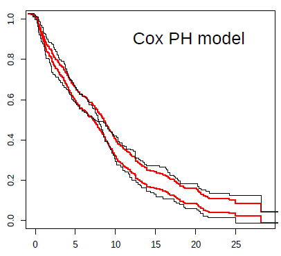
For example, in the case of the Keynote-061 trial, I show a plot with the prediction from the Cox model (in red) against Kaplan-Meier estimates (black). The inability to capture the real effect of immunotherapy in this scenario is very striking. The reason for bias and reduction in statistical power can be clearly seen in this plot. Not being taught this, the next clinical trial in an almost similar population, with the same strategy, repeated the same statistical plan. Both trials were declared negative, despite the fact that immunotherapy possibly offers great benefit to some patients with gastric cancer.

kn061

1 Like

Add to the plot the confidence and for the difference in the two curves, which would better support your implication that there is signal there that a PH model missed.

3 Likes

I was curious and made the analysis you suggest, for the Keynote-061 trial… the authors considered it negative, literally concluding that pembrolizumab does not increase overall survival.
https://www.thelancet.com/journals/lancet/article/PIIS0140-6736(18)31257-1/fulltext
Instead, on this plot, I show the difference of survival with the survdiffplot function of the rms package.

This is the same conclusion as in figure 4 of our article with a spline-based model.

Sadly, because these studies have been declared negative, patients do not benefit from these strategies. Worse, clinicians don’t discuss the problem of crossing hazards. However, among my colleagues I have received quite a lot of criticism. The opinion of the clinicians is that to reanalyse clinical trials, even if they are poorly designed, is always to go fishing for p-values. So it has occurred to me to reproduce these analyses with a Bayesian Royston-Parmar model, which does not require pre-specifying the time point at which the survival difference is measured. The question would be how to pre-specify the prior for the number of parameters of the splines… Another Bayesian option would be the equivalent of survdiffplot My idea is to propose to completely abandon frequentist hypothesis tests, which lead to a dead end.
Instead, a Bayesian estimate of survival differences could be shown with their credibility intervals at all points at once. Instead of a decision criterion, the clinician could qualitatively judge the entire curve. I think this goes in the direction of the spirit of times. The FDA is actually accepting promising drugs only with phase I/II trials in orphan indications. So the Bayesian analysis would explicitly address this real concern of the regulators.

2 Likes

The graphic above conveys something nice for me. By not capturing the crossing curve as expected, the differences in survival predicted by Cox’s model for late time points are biased, being smaller than the real ones. This beautifully illustrates, in my oncological opinion, the loss of statistical power that you risk if you use Cox’s model for this data. If you add the super convoluted hierarchical designs, it is almost impossible that any of these trials could be positive.

1 Like

Really nice displays that give ammunition that the PH assumption really mattered here.

You raise some huge points that should be discussed for a while. Regarding trustworthiness of reanalysis, I’m feeling more and more that if we use self-penalizing approaches we should be granted leeway. A rational approach that is self-penalizing is having 2 parameters for treat: treatment main effect + tx by log(time) interaction. Then estimate treatment effect as a function of time with highest posterior density intervals.

This begs the question of which treatment is better. That depends on the patient’s utility function. There is no single answer. But presenting results for all times (whether log hazard ratio vs. time or differences in cumulative incidences) is a great way to communicate this.

5 Likes

For many oncologists one of the most bizarre passages in the history of medicine occurred in this article:


Mok et al wrote:
The median progression-free survival was 5.7 months in the gefitinib group and 5.8 months in the carboplatin–paclitaxel group […]. The study met its primary objective of demonstrating noninferiority and showed the superiority of gefitinib as compared with carboplatin–paclitaxel for progression-free survival […]. Apparently they published in NEJM that 5.7 is more than 5.8 months.

Here, beyond the analysis, the important thing is that the crossing hazards always translate the presence of a strong effect-modifying factor. In the case of Mok et al, EGFR mutations. For immunotherapy there is certainly a strong predictive factor yet to be discovered, which is fascinating.

If I understood correctly, you suggest using the formula treatment + treatment * time in a survival model. That could work for non-PH scenarios.
My doubt is how to code the crossing hazards with only two degrees of freedom. My experience with the Royston-Parmar model was that 5+5 degrees of freedom were required to capture the behavior of the more complex examples. Below I show the plots we made by comparing the model estimates with the KM curves. With less degrees of freedom the Royston-Parmar model, which is quite flexible, worked quite worse. If you look at it, the curves do some really weird things.

4/2 is looking pretty good. If you used a Cox PH model you should be able to get by with a simple 1 d.f. interaction with time (but only if time were properly transformed in the interaction term).

Frank, I’m not sure that with a single parameter I can capture an interaction with morphology as complex as the KM curves above. If you can be more precise with the formula you suggest, I’ll try.

We may know more if you plot the curves on the log relative hazards scale (log(-log(S(t)))).

This is the plot…

The point is that each curve has a different morphology, with more or less serious violations of the proportional hazard assumption, and with different fluctuations of the risk. The question is how to model them all with a single pre-specified formulation. The spline-based model picks them up very well but sometimes requires many degrees of freedom to do so. The question is how to pre-specify it in a simple way. You sometimes talk about using Bayesian methods, with priors that favor simple models with few degrees of freedom, but allow more complex models if needed. Perhaps it would make sense to use hyperpriors for the degrees of freedom of the splines, in a hierarchical way…

1 Like

Yes a hierarchical way of thinking is really good. But I’m seeing a fairly linear relationship between log t and the difference in those two curves, so maybe I’m missing your point. In the Cox model we don’t care about the shape of any one of the two curves.

If you can compute the vertical differences between the two curves that would tell is if what I saw is an optical illusion.

1 Like

I have computed the difference between the two arms of the log(-log survival ) vs log(time) plot above. This is the code and the result… so?

survi<-summary(survfit(sur~arm, data = kn061), time=seq(1,28,0.1 ) )
survi$surv=log(-log (survi$surv))
survi$time=log(survi$time)
survi2<-data.frame(strata=survi$strata, time=survi$time, surv=survi$surv)
s0<-survi2[survi2$strata=="arm=1",]
s1<-survi2[survi2$strata=="arm=0",]
survi2$diff= s0$surv- s1$surv
ggplot(data=survi2, aes(x=time, y=diff)) +
        geom_line()

2 Likes

As I guessed, the interaction between log(t) and treatment effect is linear so should be easy and efficient to model treatment with a total of 2 d.f.

1 Like

Ok, so I’m going to fit the model, and then represent its predictions vs Kaplan-Meier. What would the formula be then, arm + arm * log(time)??

1 Like