Marginal vs conditional (Mixed) models used in Joint model analysis. The SPRINT trial controversy

Dear Colleagues, this is an update to the academic discussion posted on datamethod.org
regarding a secondary analysis of the SPRINT trial(1) did by our research group in Erasmus University Medical Center.[https://journals.lww.com/jhypertension/Fulltext/2019/05000/Impact_of_cumulative_SBP_and_serious_adverse.24.aspx] The core of this post is based on an editorial letter written by Dr. Reboussin and Dr. Whelton (main researchers of SPRINT trial) discussing our methodological approach and results(2) https://journals.lww.com/jhypertension/Citation/2019/08000/Joint_modeling_of_systolic_blood_pressure_and_the.25.aspx. I want to divide this introduction to the discussion into three parts:

1. Why applying joint models for longitudinal and to time-to-event data analysis to SPRINT trial?

The main aim of SPRINT trial(3) was to evaluate if an intensive treatment approach ( lower SBP below 120 mmHg) compared with standard treatment ( maintain SBP between 135-139 mmHg) decrease the hazard to the composite SPRINT primary outcome (Myocardial infarction, other acute coronary syndrome, heart failure, stroke and cardiovascular mortality). The traditional Cox model analysis was the statistical method used in the original SPRINT trial.

SPRINT trial measured systolic blood pressure (SBP) monthly in the first trimester and then every quarter for 3.26 years median follow-up (range 0 to 4.5 years), in 9361 participants, achieving an average of 15 SBP measurements per person (range: 1-21) during follow-up. This information was not taken into account in the primary SPRINT analysis. Given that: (i) this clinical trial evaluates a strategy of intensive pharmacological intervention (decreasing the SBP <120 mmHg) versus conventional treatment (SBP between 135-139 mmHg), (ii) blood pressure is among the most important risk factor for major cardiovascular events (primary SPRINT outcome), (iii) there is a high SBP variability within the subjects during follow-up (figure 1)

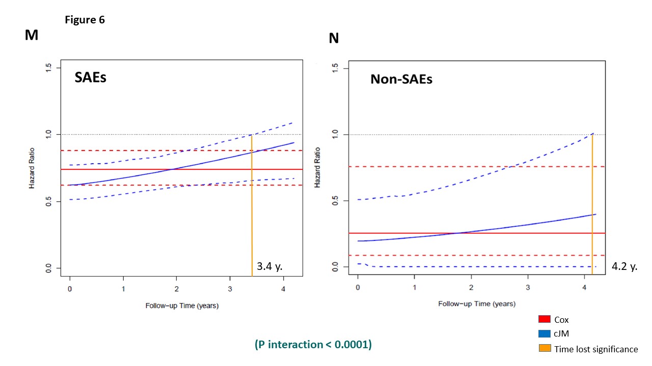
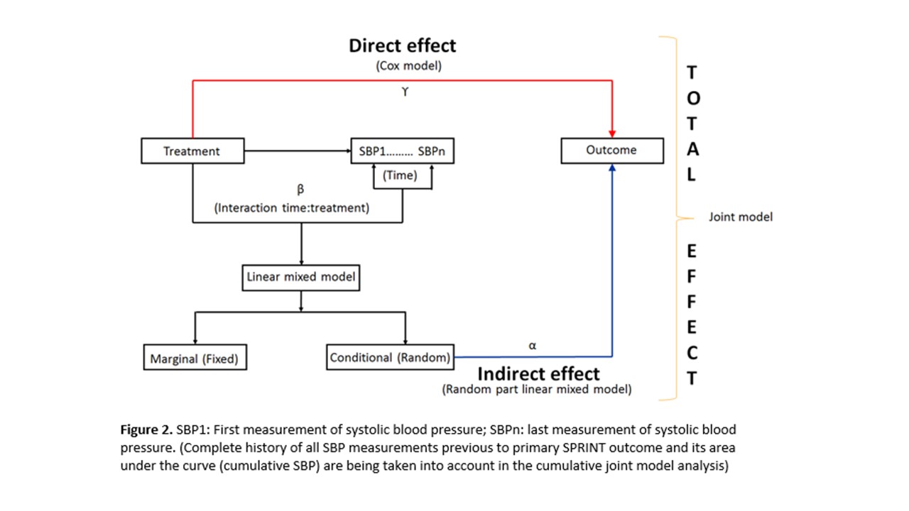
, and (iv) the occurrence of serious adverse events (SAEs) during follow-up can impact both the subsequent SBP figures as well as the primary outcome; a statistical analysis is required that evaluates the impact of longitudinal changes in SBP both within individuals and between intervention groups and takes also the cumulative effect of the SBP on the primary outcome into account (Indirect effect) + the effect of this intervention in the primary SPRINT outcome (Direct effect). This analysis can only be achieved with a statistical model that includes all these elements at the same time, such as the cumulative joint model (cJM) analysis (Figure 2).

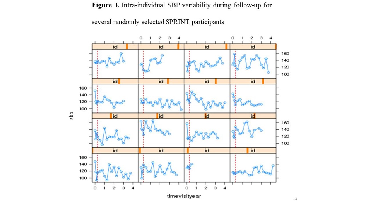
2. Criticisms of Dr. Rebousssin and Dr. Whelton to our SPRINT secondary analysis (2)https://journals.lww.com/jhypertension/Citation/2019/08000/Joint_modeling_of_systolic_blood_pressure_and_the.25.aspx.

The main concern from Dr. Reboussin and Dr. Whelton to our secondary analysis could be summarized as:

  • Analyses of clinical trials that adjust for variables measured after randomization estimate something very different than standard clinical trial analyses which do not employ adjustment or only adjust for baseline variables
  • Rueda-Ochoa et al. make a serious error in defining the ‘total treatment effect’ as one that ‘accounts for differences in SBP over time’. In fact, what they report is the component of the intervention effect that excludes the effects produced by changes in SBP. This cannot be viewed as a complete summary of the intervention effect. At best, estimation of this adjusted effect represents a technical accomplishment without clear implications for clinical decision-making.
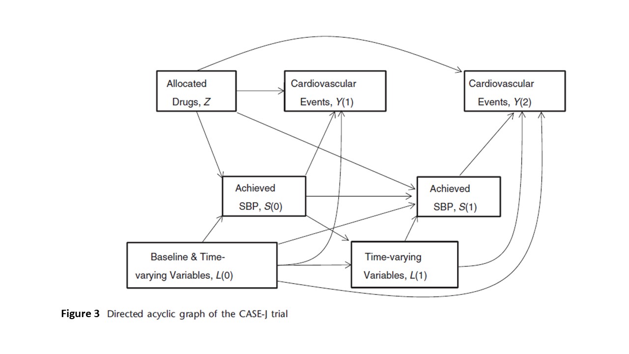
  • The Rueda-Ochoa et al secondary SPRINT analysis is similar to the CASE-J trial reported by Oba paper previously published(4) https://www.ncbi.nlm.nih.gov/pubmed/21730076 (Figure 3)
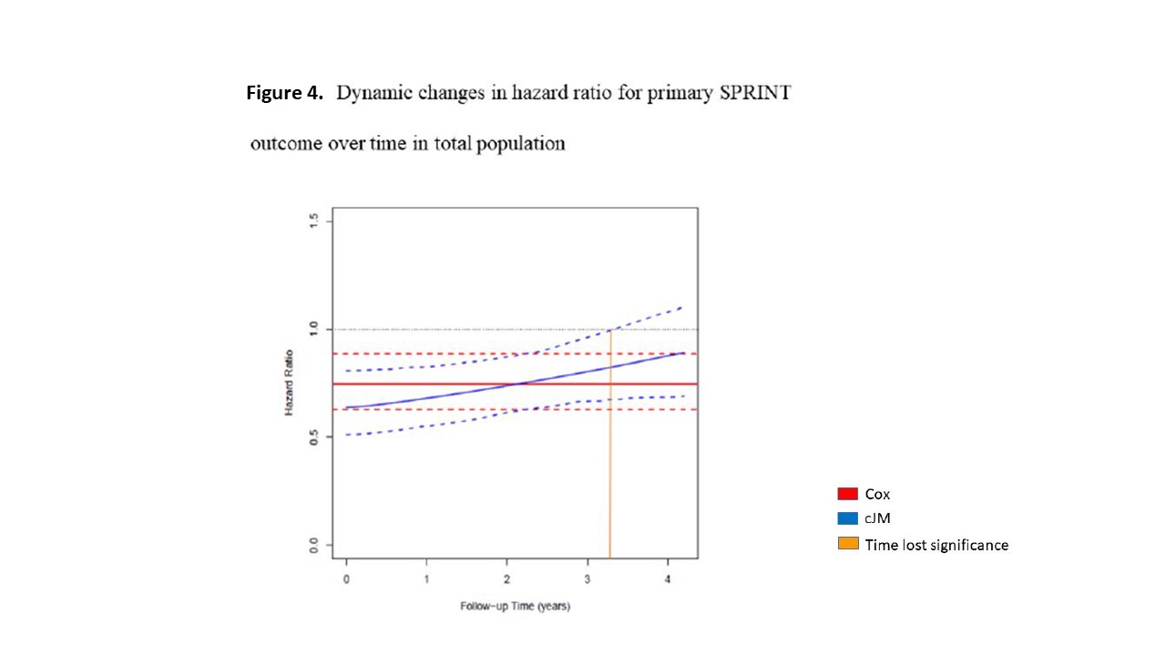
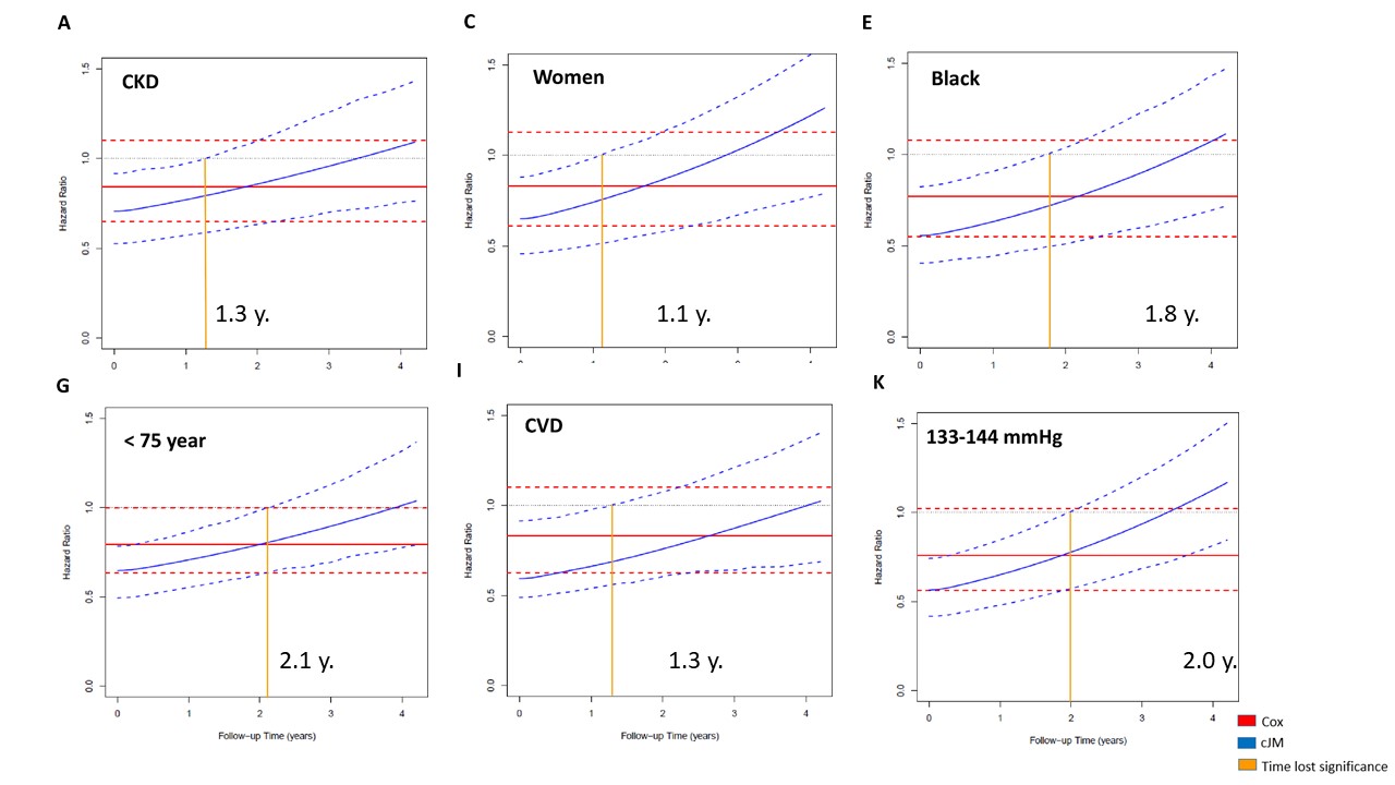
  • Compared with the standard intervention, the SPRINT intensive intervention resulted in substantial health benefits, including prevention of CVD events, total mortality, and cognitive impairment that were, if anything, larger later in the follow-up period rather than smaller, as suggested by Rueda-Ochoa et al.

3. Our Reply to Dr. Reboussin and Dr. Whelton editorial letter (4)https://journals.lww.com/jhypertension/Citation/2019/08000/Reply.26.aspx

  • The joint modeling approach does not condition on systolic blood pressure (SBP) after randomization but rather treats it as an outcome. In particular, the joint model uses a linear mixed model for SPB that explicitly allows for different SPB profiles in the two treatment groups. In addition, among others, it accounts for the correlations in the repeated SBP measurements per patient, for missing at random missing data, and the endogenous nature of SPB that relate to the challenges in the interpretation mentioned by Dr. Reboussin and Dr. Whelton.

  • The total effect we have report is the sum of both direct and indirect effect of the intervention. (Figure 2)

  • Our cumulative Joint model analysis is not similar to CASE-J trial analysis in which was used a marginal approach. We used a conditional (mixed ) model approach + Cox proportional hazard model = Joint model analysis. For more detail comparison between these approaches, I recommend Lindsey Jk and Lambert P. paper https://www.ncbi.nlm.nih.gov/pubmed/?term=STATISTICS+IN+MEDICINE%2C+VOL.+17%2C+447%C3%90469+(1998)+Statist.+Med.%2C+17%2C+447%C3%90469+(1998)

  • It should be remembered that in the cumulative joint model analysis one takes into account the effect of SBP (cumulative and intra-individual SBP variability) on primary SPRINT outcome and it is not only the marginal difference in events. Clearly, the differences found in the changes over time in the HR in our analysis compared with the number of events marginally reported by Whelton et al can be along the lines of Yule-Simpson´s paradox.

Finally, I would like to invite to all colleagues to contribute in this academic discussion.

4 Likes

thanks for updating us on this topic. I’d say, off the bat, that i agree with your response (summarised above), and your modelling approach. I also agree with the need for ongoing discussion: I feel it is a good thing that the data are being analysed in different ways, even if this is leading to conflicting conclusions and prolonging discussion. Eg, net benefit is difficult to define

to be honest, I’m perplexed by the letter from the biostat and epidem who misunderstood your modelling approach. I have moaned before on this message board about the inappropriate use of terms “multivariate” and “multivariable”. With tongue in cheeck i might speculate that it is because these terms are applied to everything-under-the-sun that people cannot detect actual multivariate data when they are confronted with it

you mention eg the “impact of SAEs on the sustainability of treatment benefit over time”. Given how the data evolve over time i feel they’re in need of a visual to get a sense of what’s happening, and this might inform the analysis. Sankey plots are used to illustrate patient trajectories, maybe it is crude but useful: https://bl.ocks.org/micahstubbs/ed0ae1c70256849dab3e35a0241389c9

but i would like to re-read your original paper and dig into some other references and then respond further …

2 Likes

First, as an early adopter of JM (who had to battle 5 years for a JM paper to be accepted), I congratulate you for doing this. However, I am not entirely sure I agree about the interpretations of your analysis. In particular, the overall TE in a JM will never be any different than the one computed with the Cox model (assuming the usual square root asymptotics in the large samples) and your analysis confirms that. It is precisely this analysis that is central for policy, and as much as I find the SPRINT problematic to apply clinically we have to live with it.
The crux of your analysis is that a) the TE is highly heterogeneous b) it is ripped by people who do not have suffer SAE and c) non-proportionality (which due to higher power is detectable more readily with JMs) may be a clue to treatment effect heterogeneity. Needless to say, hypertension is not different from any disease in that regards: to put it more crudely, patients with cancer who can’t tolerate their oncological regimens die from cancer disease because they can’t be treated, and this is what you found for hypertension too.

From a technical perspective, I totally agree with you about JMs: this is how biomarkers of response should be analyzed :slight_smile:

1 Like

it depends on the scenario, eg with recurrent events rogers and pocock compared an assortment of models including cox for time-to-first and a joint frailty model incorporating death and concluded: “We advocate the use of the joint frailty model, as this method allows estimation of a treatment effect for recurrent events, whilst accounting for death as informative censoring.” It seems easy to predict that, analogous to ignoring recurrent events, ignoring the sbp data and running basic cox of time-to-first (by default) would lead to re-analyses and ‘controversy’. Researchers should try to pre-empt this

Dr. Brown, thank you for your comments. Our main result, using a cumulative joint model analysis, was that when the cumulative effect of having a SBP lower than 120 mmHg over time is taken into account, the beneficial effect of intensive treatment is lost after 3.4 years of follow-up. Figure 4 shows the graphs of the dynamic changes in the hazard ratio over time (comparing the intensive treatment versus the standard treatment on the primarySPRINT outcome ) using the analysis of the cumulative joint model versus the traditional Cox proportional hazard analysis, used in the original SPRINT analysis.

This loss of the protective effect of intensive treatment on the primary outcome of SPRINT occurred early and similarly, mainly in women, black participants, participants with a history of chronic kidney disease or cardiovascular disease, under 75 years of age and participants with a SBP greater than 132 mmHg at the beginning of the study. Figure 5

What could be the cause of the loss of protection from intensive treatment over time? We suggest two explanations:

  1. Serious adverse events (SAEs): Although the amount of SAEs was similar in both intensive and standard treatment, the SAEs produced by the intensive treatment increases the risk of primary SPRINT outcome 3 times more than the SAEs in the standard treatment because they were more severe. (Higher acute kidney injury, electrolyte abnormalities, hypotension, and syncope) Figure 6 shows the dynamic changes in the hazard ratio by comparing intensive versus standard treatment on the primary SPRINT outcome in participants with and without SAEs.

  2. Greater variability of SBP produced by intensive treatment. We found significantly greater variability of SBP in the participant who received intensive treatment compared to the standard treatment group. It has been reported that greater SBP variability is associated with an increase in major adverse cardiovascular outcomes.

Finally. I agree with you that the data must be analyzed in different ways. This concept called triangulation is well explained by Davey Smith et al.https://www.ncbi.nlm.nih.gov/pubmed/28108528 The question is: what additional methods could we use to try to confirm our findings? I would like to hear the opinions of our colleagues on this question.

3 Likes

Dr. Argyropoulos, thanks for your comments. To put the problem in context, I would like to mention that multiple epidemiological evidence based on clinical trials and observational studies have shown that hypertension is the main modifiable risk factor related to major adverse cardiovascular outcomes. Dr. Pfeffer makes an excellent review of clinical trials that have led to the definition of the target for the proper management of hypertension. https://www.nejm.org/doi/10.1056/NEJMra1510067?url_ver=Z39.88-2003&rfr_id=ori:rid:crossref.org&rfr_dat=cr_pub%3Dwww.ncbi.nlm.nih.gov

Given that a decrease in blood pressure levels is accompanied by a cardiovascular protective effect, it has been decided to evaluate whether further decreasing the blood pressure figures provide additional benefits of cardiovascular protection, this is the main reason for the SPRINT study. Our findings, using the original database of this study, showed that intensive treatment reduces the risk of major cardiovascular events, as shown by the original SPRINT study; however, such protection does not hold up over time in the total population and especially in certain subgroups, as I mentioned in a previous comment. In addition, the early loss of protection in certain subgroups, has a clear tendency to increase cardiovascular risk in them, forces us to reassess whether such intervention can be considered a universal recommendation that guides our usual clinical practice. I am not totally in agreement with your example between oncology and hypertension, since a patient in whom the intensive treatment is not indicated or does not tolerate it, has the option of receiving the standard treatment that has also shown benefits in the reduction of cardiovascular risk .

Given your previous experience in join model analysis, I would like to know your opinion about the role that this type of analysis can play in the design of new clinical trials and if you consider that the FDA should include this analysis and others that involve time-varying covariates, for the evaluation of the effectiveness of health interventions.

2 Likes

Questions to the audience

Dear Profesor Harrell and colleagues, I would like you could contribute to this academic discussion sharing your opinion about these two questions:

  1. What additional methods could we use to try to confirm our findings of the Joint modelling SPRINT secondary analysis?

  2. I would like to know your opinion about the role that Joint modelling analysis can play in the design of new clinical trials and if you consider that the FDA should include this analysis and others that involve time-varying covariates, for the evaluation of the efficacy of health interventions.

To elucidate the apparent contradictions between the original SPRINT report and Rueda et al.’s findings we need to keep in mind what was the target (causal) parameter estimated in both studies. The standard intention to treat analysis used in the SPRINT trial aimed to estimate what is the marginal causal effect of intensive treatment (T1), as compared to regular treatment (T0), on cardiovascular outcomes (Y), among hypertensive patients. A marginal effect in this case responds to the clinically relevant question of what is the best treatment option we could offer our patients (i.e. patients similar to those enrolled in SPRINT). By creating exchangeable treatment groups, i.e. groups with asymptotically equivalent potential risk of Y, randomization, followed by intention to treat analysis, provides a valid (unbiased) estimate of the effect of T1 on Y. From the point of view of estimating causal effects, it is irrelevant how the T1 excerpts its effect on Y. In other words, in the case of the SPRINT trial, it is irrelevant if the effect of intensive treatment is due exclusively to a decrease in blood pressure (BP), exclusively to non-BP related mechanisms, or to both BP- and non-BP mediated effects. The causal effect of T1 on Y would be valid and would remain unchanged, regardless of its mechanism.

Rueda et al.’s found that indicate cumulative systolic BP (SBP) and development of treatment-induced serious adverse effects (SAEs) might offset an initial benefit of T1 during follow-up. This suggests their target (causal) parameter differs from that in the original SPRINT trial. They showed that the effect of T1 on Y changed after the first 4 years of follow-up, depending on the presence of SAEs. Thus, they were interested in conditional effects. Even if we assume their findings are valid, they do not invalidate the original findings of the SPRINT trial. It is perfectly possible for a treatment to have different effects in different subpopulations. For instance, vitamin A supplementation would reduce mortality in children with vitamin A deficiency, but not in those without deficiency. Therefore, a marginal effect in a given population would depend on the proportion of children with and without vitamin A deficiency, and may be different from the conditional effect in each group. Although this example does not corresponds exactly with the case in question, it shows we should expect marginal and conditional effects to differ in specific settings.

Rueda et al. estimated the effect of T1 on Y in patients with and without SAEs and found it was different in patients who developed SAEs, but only after about four years of follow-up. The frequency of all SAEs in the original SPRINT report was similar in both treatment groups. In contrast, in Rueda et al.’s analysis, specific SAEs were more frequent in the T1 group (as shown in their Table 2) and among patients who developed the outcome (Y). This discrepancy should not be surprising because the original SPRINT trial included SAEs that were not necessarily a consequence of intensive treatment (such as an injury resulting from a fall). Some SAEs, such as syncope (SY), could be both a consequence of the treatment and an early manifestation of one of the components of the outcome (say stroke). Conditioning on such variables (colliders) results in selection bias, regardless of the approach used for conditioning (stratification, Cox regression, joint modelling, etc.). This is one of the reason why conditioning on variables measured after treatment assignment is not recommended in the analysis of randomized trials. If SY were a consequence of T1, but not a consequence of Y, we would not need to adjust for SY, because it would not be a confounder. If SY were a consequence of Y, but not a consequence of T1, it would not be a confounder, and adjustment for SY would not be needed. If SY were a consequence of T1 and in turn increased the risk of Y (i.e. were a parent of Y), then SY would be a mediator of the effect of T1 on Y. In that case, adjusting for SY would nullify the proportion of the effect of T1 on Y that is mediated through SY. This would result in a biased estimate of the effect of T1 on Y. This also applies to SBP, regardless of how the trajectory of SBP is modelled. Briefly, conditioning on SAEs and/or SBP will bias the estimate of the effect of T1 on Y.

If SAEs were colliders negatively or positively correlated to both T1 and to Y, adjusting for them would introduce selection bias towards the null. This bias would happen in both patients with and without SAEs. In other words, the measured effect of T1 on Y will be weaker than the true effect in both patients with and without SAEs. SAEs accumulate with time. Thus, the selection bias only happens after some time. This could explain the weakening of the beneficial effect of T1 on Y with the passing of time in Rueda et al.’s analysis.

Another limitation of the JM analysis in this case is that the number of outcome cases in individuals without SAEs was only 20. Such a small number of cases could have resulted in sparse data bias. In the regression models, these 20 individuals would have to be distributed into eight cells defined by four time groups (knots) and two treatments, compromising the stability of the model. Indeed, the large estimate of the effect of treatment in this group (hazard ratio of 0.19) and the wide confidence interval (0.06, 0.63) suggest sparse data bias.

I am not familiar with joint models (JM). I believe they were developed as an option to including time-dependent variables (TDVs) in a Cox regression model. They seem useful when the TDV was a continuous variable, such as SBP in this case. By using JM, one can take advantage of the variability in the measurement of the TDV (i.e. better account for error in the measurement of the TDV). I have the impression TDVs included in early JM were not a consequence of the exposure (T1). Although SBP was used as an outcome in the linear mixed sub-model of the JM, fitted values of the predicted SBP (i.e. the SBP trajectory) were included in the Cox model for the effect of treatment on survival. Therefore, estimates of the effect of T1 on Y from the JM were likely biased towards the null.

If the continuous variable used as outcome in the linear mixed model were not a consequence of the treatment, randomization would result in a balanced distribution of its values at baseline and during follow-up (assuming balance in co-intervention and non-differential measurement error). An instance of such a TDV would be LDL-cholesterol. If we were interested on the effect of the trajectory of LDL-c on Y, using SPRINT data, JM could offer some advantage over Cox-regression. However, the effect of T1 on Y will be the same in both models (disregarding precision), because the effect of T1 is not mediated through LDL-c. In consequence, JM would offer little advantage over Cox-regression, when the target parameter is the causal effect of T1 on Y. Indeed, in the case of LDL-c the JM will reduce to two standard models, because T1 does not affect LDL-c levels: a mixed model for LDL-c and a Cox model for Y (see Ibrahim DOI: 10.1200/JCO.2009.25.0654 and Crowther: The Stata Journal (2013) 13, Number 1, pp. 165–184).

Of course, JM could be used to estimate the direct and indirect (mediated) effects of T1 on Y. In other words, JM could be used to estimate to what degree the effect of T1 on Y is due to changes in SBP, and to what degree is due to other mechanisms. Under strong assumptions, we could use the direct and indirect effects from JM to estimate the total effect of T1 on Y. As a simplification, the total effect of T1 would be the sum of its SBP-mediated effect and its direct effect. For this purpose, one needs to estimate the effect of T1 on SBP and the causal effect of SBP on Y, to obtain the indirect (mediated) effect of T1 on Y. A model with treatment and time would suffice to estimate the effect of T1 on SBP, because all other variables that influence SBP will be balanced, thanks to the random assignment of the treatment. Estimating the effect of SBP on Y would be more complicated, because we would need to control for variables that confound the SBP-Y association. Unfortunately, confounders of the SBP-Y association are not controlled through the randomization, because it is the treatment and not SBP that is assigned at random. SBP-Y confounders were not included in Rueda et al.’s joint models. Most likely, those confounders were not measured in SPRINT, because they are not needed to estimate the causal total effect of T1 on Y. Thus, in Rueda et al.’s analysis, the mediated effect was likely biased. This problem may have been compounded if some SBP-Y counfounders were also a consequence of the treatment. As far as I know, JM cannot account for these confounders. Since the effect of the mediator (SBP) on Y will be likely bias, the indirect effect and the total effect of T1 on Y will be biased.

JM may provide some advantage over a stratified Cox model when estimating the effect of a TDV on an outcome. However, it does not seem to provide any advantage for estimating the effect of a treatment on an outcome in the context of a clinical trial. JM estimate the total effect of the treatment by way of a mediation analysis that requires strong assumptions. Some of those assumptions are untestable, and none is required in a standard Cox regression analysis.

From a clinical perspective, if T1 offers a substantial benefit, we should offer it to our patients, even if the benefit only lasts four years. After all, during the first for years of treatment, the risk of Y will be 30% lower in patients receiving intensive treatment. Of course, we should also take into account the risk of SAEs while making this offer. In contrast, we should not take into account changes/trajectory in SBP, since they have little or no weight on this decision. Therefore, the key information to make this is which treatment option would be best, in average, considering beneficial and harmful effects. An answer to this question was provided by Richman et al. (doi:10.1001/jamacardio.2016.3517), who showed that intensive blood pressure management is cost-effective among US patients with hypertension at high risk for cardiovascular disease.

2 Likes

Thanks for all the discussions. Lbautista’s posting is really instructive for me. At first, in terms of interpretation, mediator idea seems to be useful to understand the story behind even though the formal analysis is not allowed due to strong assumption as noted by Lbautista. JM could only provide the way of looking at SBP in SPRINT as a sort of one of the mediator for the outcome.

Due to the controversial results obtained in this secondary analysis of the SPRINT study, new analyzes are required, using other statistical approaches to validate our results. (Triangulation approach). In this sense, Rizopoulos et al have recently published a new analysis of the effect that SAEs have on the composite outcome of the SPRINT study, using a more flexible joint model and reaching similar conclusions.

https://onlinelibrary.wiley.com/doi/full/10.1002/sim.8387

https://onlinelibrary.wiley.com/action/downloadSupplement?doi=10.1002%2Fsim.8387&file=SIM_8387-Supp-0001-Supplementary_Material+(SIM-18-0316_R2).pdf

Finally, I want to insist that The joint modeling approach does not condition on systolic blood pressure (SBP) after randomization but rather treats it as an outcome in the linear mixed model. So, SBP is not considered a classical mediator (Figure 2 in this forum discusion).

3 Likes