Should one derive risk difference from the odds ratio?

Following up on citations to that arXiv paper lead me to a valuable series of relatively recent papers that discusses this effect measure issue from a public health and program evaluation perspective that will clarify why collapsible effect measures are important in this application.

From the author reply, they make the following claim:

  1. The odds ratio is not a parameter of interest in epidemiology and public health research. 5 Instead, the relative risk and risk difference are two often-used effect measures that are of interest. Both of them are collapsible. Directly modeling these two measures6,7 eliminates the noncollapsibility matter entirely.

They cite the following paper by Sander:

Greenland, S. (1987). Interpretation and choice of effect measures in epidemiologic analyses. American journal of epidemiology, 125(5), 761-768. (PDF)

I will argue only incidence differences and ratios possess direct interpretations as measures of impact on average risk or hazard … logistic and log-linear models are useful only insofar as they provide improved (smoothed) incidence differences or ratios

Would you mind if I started a new thread, similar to the wiki-style Myths thread, that summarizes the areas of agreement in this one, along with references to the relevant literature? I think it is time to put the relevant issues – higher level clinical questions and the statistical modelling and reporting, in a decision theoretic framework.

After following up on a number of citations, I get the feeling that researchers are still hampered by traditions that were somewhat reasonable given the space and computational constraints of the past, but are not aware that we can do much better with modern computing power.

Relevant Reading:

Greenland, S., & Pearce, N. (2015). Statistical foundations for model-based adjustments. Annual review of public health, 36, 89-108. (PDF)

Here is a recently updated version summary (March 2023) of the @AndersHuitfeldt paper on the switch risk ratio.

For a statistical justification of the switch (causal) relative risk, the following is worth study:

Van Der Laan, M. J., Hubbard, A., & Jewell, N. P. (2007). Estimation of treatment effects in randomized trials with non‐compliance and a dichotomous outcome. Journal of the Royal Statistical Society: Series B (Statistical Methodology), 69(3), 463-482. https://rss.onlinelibrary.wiley.com/doi/abs/10.1111/j.1467-9868.2007.00598.x

We will show that the switch causal relative risk can be directly modelled in terms of (e.g.) a logistic model, so that the concerns expressed above for modelling the causal relative risk [ needing to correctly specify nuisance parameters] do not apply to this parameter.
1 Like

That is not my main paper on the switch relative risk, just a short summary that was published recently in Epidemiology, in order to bring attention to the history of this idea, and in particular to the contributions of Mindel C. Sheps, who died 50 years ago this year.

My original paper on the switch relative risk (which did not use that term, but contained most of the relevant ideas) was too long for epidemiology journals and was therefore split up into three separate papers and published as The Choice of Effect Measure for Binary Outcomes: Introducing Counterfactual Outcome State Transition Parameters (which contains the methodological considerations for choosing between effect measures), Effect heterogeneity and variable selection for standardizing causal effects to a target population | SpringerLink (which contains my argument for why effect measures are still necessary; this is something that some people in the causal inference community need to be convinced about, but most people in this thread are probably on the same page as me on that particular question) and On the collapsibility of measures of effect in the counterfactual causal framework | Emerging Themes in Epidemiology | Full Text (which introduces some collapsibility weights that were used in the other papers)

After those papers were published, I became more familiar with some of the relevant older literature, and started using more standard terminology. I subsequently wrote [2106.06316] Shall we count the living or the dead? , which probably contains my most complete and most convincing attempt to make this argument. This manuscript does not really introduce much new theory that wasn’t already contained in the three papers above (other than a demonstration that the same argument can be made with causal pie models, and a new impossibility proof for why it is impossible for certain types of data generating mechanisms to result in stability of a non-collapsible effect measure) but if someone wants to understand my point of view, it is probably where they should start.

1 Like

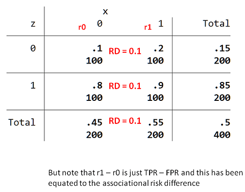
Anders: I think if we look back at Doi’s last post you and I may agree that it doesn’t correctly grasp the targets in the potential-outcome (counterfactual) causal models underlying our recent discussions and those in older papers such as Greenland-Robins-Pearl Stat Sci 1999. To tie the switch-RR (SRR) to the type of two-stratum OR-noncollapsibility examples in which the OR and RD are both constant, I would ask if you would display the SRR for an example in which there are two strata of 100 patients each, and in stratum 1, 90 die if treated but 80 die if untreated, while in stratum 2, 20 die if treated but 10 die if untreated. If I have not made an error, the causal RD is 0.1 in both strata as well as marginally (the causal RD is strictly collapsible), while the causal OR is 2.25 in both strata but the marginal causal OR is about 1.5 (the causal OR is not collapsible). The causal RR is collapsible but not constant, a description which could be said to depend on the causally relevant weighting for the RR. It may be worth noting that these results depend only on the stratum-specific marginal distributions of the potential outcomes, thus avoiding the objections to positing a joint distribution for them, and so they carry over when using instead certain decision-theoretic causal models.

My question for you is how you would describe the behavior and weighting of the SRR in this example and more generally, given the causal model.

1 Like

I assume you mean two strata of patients with 100 in each of the treated and untreated groups……
In that case we have the following results:

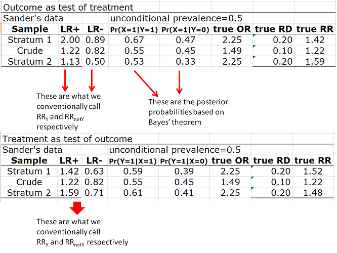
As can clearly be seen the LR is being mistaken to be the RR and this to me seems to be the basis of all the controversy around noncollapsibility. Obviously, in stratum 1, if we apply a baseline probability of 0.5 (keep in mind that a baseline probability is a conditional probability) then the RR derived predicted probability is 1. This does not make sense to me and does not align with Bayes’ theorem. The mistake all along has been not recognizing that the RR is actually a LR and treating it as an effect measure. Of course, I am happy to be corrected based on any detected mathematical issues but not if based on imaginary mechanisms of generation of data.

NB: I renamed ‘baseline probability’ to ‘unconditional prevalence’ in the tables to avoid misunderstanding. In the top panel the prevalence is of treatment ‘X’ while in the bottom is of outcome ‘Y’

Great idea. But beware - I have the suspicion that some of those papers make the mistake of implying you should directly model RRs and ARRs instead of getting them from a proper probability model.

I have been trying with some difficulty to follow your discussion @sander, @s_doi and @AndersHuitfeldt about collapsibility of the proportions in @s_doi’s tables.

It is my understanding that RR is collapsible when r is constant under the following circumstances: p(Y=1∩X=0|Z=1∩X=0)/p(Y=1∩X=1|Z=1∩X=1) = r, p(Y=1∩X=0|Z=0∩X=0)/p(Y=1∩X=1|Z=0∩X=1) = r and the marginal p(Y=1∩X=0|X=0)/p(Y=1∩X=1|X=1) = r. This situation will arise in the special case when p(Z=1∩X=1|Y=1∩X=1)=p(Z=1∩X=0|Y=1∩X=0) and also if p(Z=1∩X=1|X=1)= p(Z=1∩X=0|X=0). It follows that the ratios of ‘survival from Y=0’ (i.e. Y=1) will also be collapsible. These special cases will be met rarely in a precise manner for observed proportions that are subject to stochastic variation and can only be postulated for ‘true’ parametric values.

It is also my understanding is that the OR will be collapsible when r’ is constant under the following circumstances odds(Y=1∩X=0|Z=1∩X=0)/odds(Y=1∩X=1|Z=1∩X=1) = r’, odds(Y=1∩X=0|Z=0∩X=0)/odds(Y=1∩X=1|Z=0∩X=1) = r’ and the marginal odds(Y=1∩X=0|X=0)/odds(Y=1∩X=1|X=1) = r’. It follows that the odds ratios for Y=0 will also be collapsible. This collapsibility of odds will arise in the special case when p(Z=1∩X=1|Y=1∩X=1)= p(Z=1∩X=0|Y=1∩X=0) and p(Z=1∩X=1|Y=0∩X=1)= p(Z=1∩X=0|Y=0∩X=0).

In the special conditions for OR collapsibility, p(Z=1|X=1)≠p(Z=1|X=0) so that when the OR is collapsible, it does not model exchangeability at baseline between {X=0} the set of control subjects and {X=1} the set of treated subjects. Therefore p(Z=1|X=1)≠p(Z=1|X=0) implies that p(Z=0|X=0) is a pre-treatment baseline probability of the covariate Z=1 and p(Z=1|X=1) is a post treatment probability. However, the RR and SRR models do model exchangeability between the sets {X=0} and {X=1}. Again these special cases will be met rarely for observed proportions subject to stochastic variation and can only be postulated for ‘true’ parametric values.

In my limited experience of analysing data for diagnostic and prognostic tests, the observed proportions remain different to the above special cases but often not too different so that it possible to assume that the data is compatible with parameters that satisfy either of the conditions for collapsibility of OR and RR.

So in conclusion I can follow your reasoning that the RD is collapsible (0.2-0.1 = 0.1, 0.9-0.8- =0.1 and marginal 0.55-0.45 = 0.1. I follow that the OR are not collapsible (2.25, 2.25 and marginal 1.5) and especially as the data do not satisfy the special case of paragraph 3 above. Regarding RRs, I find them to be 90/80= 1.125, 20/10=2 and marginal 110/90 = 1.22. In this context, what do you mean @sander by “the causal RR is collapsible but not constant”?

1 Like

Hi Huw, I think its best you look at this from the diagnostic test perspective. As Sander said and you rightly pointed out the RD in each stratum is 0.1 and the table of Y probabilities is as follows (I use X for treatment, Y for outcome and Z for the stratum variable):

However the RD is TPR - FPR and the RR is TPR/FPR in diagnostic test language and therefore RR is also the likelihood ratio. The table above therefore gives us 6 likelihood ratios (three pLR and three nLR values) and we can then compute conditional probabilities for any baseline unconditional prevalence of the outcome (or the treatment depending on how the test assignment is made). The ratios or the differences of conditional probabilities are also noncollapsible meaning that the marginal is to one side (lower) of the stratum specific effects. This only happens when the stratum variable is prognostic for the outcome and one would expect this with diagnostic tests. Only likelihood ratios are collapsible as they should be but they are not effect measures.
The above then explains the tables I posted previously. The concept of the RR as used today is therefore (as I have said previously) not consistent with Bayes’ theorem. From the diagnostic test perspective the Z strata (0, 1) and total (marginal) represent two different spectra of ‘disease’ and therefore have likelihood ratios that indicate different test performance.

Huw: A general definition of collapsibility is in col. 1 p. 38 of Greenland Robins Pearl Stat Sci 1999: “Now suppose that a measure is not constant across the strata, but that a particular summary of the conditional measures does equal the marginal measure. This summary is then said to be collapsible across Z.” Today I’d amend that slightly to “is not necessarily constant”. The particular summary here is the RR standardized to the total cohort.

1 Like

Thank you @Sander and @s_doi for your answers. I am still finding it difficult to relate the terms that you use during your explanations to my own terms and prior understanding as summarised in my previous post. For example, I think of the problem of looking at two sets – one representing control and one treatment created by randomisation and which are initially exchangeable. They change subsequently depending on the effects of treatment and control. The subsequent difference between them can be expressed in a number of ways – through RD, RR, SRR, OR or some other way. It would also help me to understand the concept of collapsibility is put into practical use. Perhaps it might be easier for you to help me if you refer to a new topic that I started a few days ago, which describes my way of thinking: Risk based treatment and the validity of scales of effect

2 Likes

Hi Huw, I think its best we continue with Sander’s example as the data is accessible to all. Also I will try to make it very clear in simple non-mathematical language so that we can benefit from your insights as an unbiased observer

First, lets assume we have three different groups based on Sander’s example:

Stratum 1 (Z=0, group 1)

Stratum 2 (Z=1, group 2)

Marginal (Mixed Z, group 3)

Since Z is prognostic for Y, these three groups represent different diagnostic test scenarios where in groups 1 and 2 the test discrimination is not influenced by Z but it is influenced by Z in group 3 (since Z is ignored).

Now consider that you would like to predict, for an individual in each group, what their probability is of having been treated based on the outcome Y=0 (or Y=1) then the best way to do this is to compute a likelihood ratio for each group – this is what I did so if we take the three groups for example:

0.2/0.1 = 2 = pLR in group 1 and 0.8/0.9 = 0.89 = nLR in group 1

0.9/0.8 = 1.13 = pLR in group 2 and 0.1/0.2 = 0.5 = nLR in group 2

0.55/0.45 = 1.22 = pLR in group 3 and 0.45/0.55 = 0.82 = nLR in group 3

Note that all the pLRs are also the RRs and now the difference emerges between what I am arguing and what causal inference groups are arguing:

My point: The RR is actually pLR and therefore TPR/FPR should be thought of as (posterior odds/prevalence odds) and should only be interpreted as such and under this constraint the ratio of posterior (conditional) risks is noncollapsible just as the odds ratio is noncollapsible

Causal inference community: It is okay to consider the TPR as treatment conditional risk and the FPR as untreated conditional risk (therefore violate Bayes’ theorem) because the benefit of so doing is collapsibility which means that the RR is now logic respecting and can be used in causal inference

I cannot see how this can work given that groups 1 & 2 above only differ on threshold not on discrimination and can therefore have different LRs but not different measures of effect. When we mix-up X with Z (marginal) we actually now have a different test scenario from groups 1 & 2 and therefore we expect here that not only the likelihood ratios but also the effect measure should be different as well and different in a consistent direction (weaker) – aka noncollapsibility albeit there is nothing bad about this anymore. This is also what Kuha and Mills tried to say in their paper which resonates with me. I look forward to your thoughts on this and to be corrected if there is any flaw of logic.

1 Like

Hi Suhail Thank you. I think that I understand. Instead of trying to predict an outcome such as death (1) conditional on treatment with S1 (e.g. with some symptom present) and control with S1 (i.e. also with the same symptom present) and (2) conditional on treatment with S2 (e.g. with the symptom absent) and control with S2 (i.e. also with the same symptom absent) and (3) conditional on treatment and control only (not knowing about S)’ you are trying to do something else. You are inverting the whole process by wishing to predict whether treatment was given conditional on the outcome (e.g. death as in a post mortem examination). In this situation, I agree with you that the risk ratio becomes the likelihood ratio since the outcome is now is whether treatment or control was given and the previous outcome (e.g. death or survival) becomes part of the evidence.

My next question is: Why should you and perhaps @sander wish to do this by predicting what has already passed? Is the ultimate purpose to try to estimate what would have happened in a counterfactual situation? Or is the ultimate purpose to try to predict the result of a RCT without having to actively randomise but instead conducting a ‘natural experiment’? I would also like to understand why ‘collapsibility’ is important in this.

3 Likes

Those are the perfect questions to raise. Backwards-information-flow conditioning is seldom useful and is dependent on more context than is forwards-time-conditioning. And I’m struggling to understand why collapsibility is interesting in any context.

1 Like

Hi Huw, I am not actually doing this inverted process by choice - I am presenting how the RR can be visualized in diagnostic terms. I too was surprised initially but this is where we stand and the RR is the LR of this inverted world-view. In other words what I am trying to say is that the RR is the LR for the ‘outcome’ as a test of the ‘treatment’ - all RRs are such LRs. In terms of the diagnostic test scenario noncollapsibility means that a prognostic covariate that has been ignored does not allow optimal assessment of ‘test’ (which is actually the outcome in a trial for example) performance until it is adjusted for - which I believe is what Frank has been saying all along.

1 Like

Frank, I agree with you, I too have reached that conclusion but some rebuttal needs to be made to causal inference groups who say its not logic respecting etc for it to be present with ORs? I am gradually moving towards the position that RR is not logic respecting but for these LR reasons. The diagnostic test scenario is one of discrimination but this is equal to association in a trial since there is no difference between the diagnostic odds ratio and the classical odds ratio.

1 Like

Hi Suhail. Would you please describe what you mean by “logic respecting”, “association in a trial”, “diagnostic odds ratio” and “classical odds ratio” perhaps using the numerical examples in your recent post.

1 Like

Hi again Sander. Would you please illustrate this explanation using the numerical examples in your discussion with Suhail @s_doi.

Hi Huw, ‘logic respecting’ means RR{z+,z−} ∈ [RRz−, RRz+] when for example there are three groups z+, z−, and all-comers {z+, z−} though I personally fail to see the ‘logic’.
The classical odds ratio is the one we are discussing and use in epidemiological studies while the diagnostic odds ratio is (tp×tn)/(fp×fn)

Huw: This has been illustrated in many articles over the past 40 years, including Greenland Robins Pearl Stat Sci 1999 and most recently here: Noncollapsibility, confounding, and sparse-data bias. Part 2: What should researchers make of persistent controversies about the odds ratio? - ScienceDirect
Please read them and their primary source citations.
See also Ch. 4 and 15 of Modern Epidemiology 2nd ed 1998 or 3rd ed 2008 for definitions of standardized measures.

2 Likes

Huw: I also strongly recommend that you (and Harrell and Doi) read thoroughly and in detail the book Causal Inference: What If by Hernan & Robins, the newest (Mar. 2023) edition is available as a free download here:

The text is searchable, so you can look up the book’s discussions of potential outcomes, counterfactuals, noncollapsibility, randomization, standardization etc.

3 Likes

Sander, this was a really good choice as a reference as the book is clearly written with all terminology explained at first use and the first part defines all key concepts in a very clear and easy to understand style and clarifies what the ‘accepted’ definitions and positions are (for the causal inference community).

In relation to the odds ratios (page 44) they however toe the same line and use personal opinion to say “We do not consider effect modification on the odds ratio scale because the odds ratio is rarely, if ever, the parameter of interest for causal inference.” There is no further information that can shed light on why this position is taken and therefore I assume its the noncollapsibility angle here too but they also do not tell us why its bad or why its ‘logic not-respecting’.

I personally think that perhaps ignoring the fact that the RR is a likelihood ratio has created this situation because LRs are collapsible but only if we ignore the pair (pLR and nLR). Had they been considered as a pair, then we are back to the OR. If we take your example data above, the outcome prevalence in the three groups is 15%, 50% and 85% and the difference between true positives and false positives (aka RD) is 0.1 because the prevalence is being ignored. If however we compute the expected r1 and r0 for the same prevalence using pLR for r1 and nLR for r0 then the RD in the same example is noncollapsible but this is being ignored. Why is it reasonable to ignore the variation dependence on prevalence?.