As I said previously we will have to agree to disagree. The justification you are making is a circular argument and simply reflects your belief that there is no violation of Bayes’ theorem for which an ex post facto justification is being made. Only a scientific analysis of why method B does not violate Bayes’ theorem should be admissible.
Hi again Suhail. Thank you - very nice! I am intrigued. So what you are saying is that there is fixed RLR ratio of 3/8 = 0.375 between odds of death conditional on treatment and control and 8/3 for the corresponding odds of survival. Conversely there is an inverse RLR of 3/8 between odds of treatment conditional on death and survival 8/3 for the corresponding odds of control. You then say that “baseline conditional probabilities may differ across different populations but RLR is variation independent”.
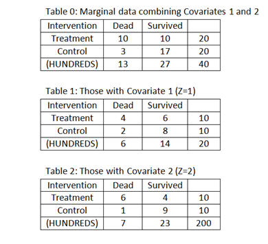
In the example with different data (see Table 0) that you gave in your rapid response [ https://ebm.bmj.com/content/early/2022/08/10/bmjebm-2022-111979.responses ], the corresponding ratios were 17/3 and 3/17. However for Covariate 1 (See Table 1 when Z=1) the ratios were 8/3 and 3/8. For Covariate 2 (See Table 2 when Z=2), the ratios were 27/2 and 2/27. This appears to show that when the baseline risks vary conditional on different covariates, then the RLRs vary too.
This appears to be inconsistent with your statement that “baseline conditional probabilities may differ across different populations but RLR is variation independent”. Perhaps that I have misunderstood again. Please advise me.
1 Like
I again see a circular argument - let me explain. You imply that methodologists do not think because they blindly follow the literature and that is a cause for concern. In that case why are you not doing the same instead of discussing on this blog? Or are you also implying that you are not in that general class you have labeled for your peers and therefore you are exempt from the same criticism?
What was circular about the argument I was making? My point is simply that Method B is nothing more than a function of probabilities. Since probabilities by definition are not quantities that can be in violation of Bayes’ theorem, it follows that Method B is not in violation/rejecting/not in the spirit of Bayes’ theorem, or however you want to put it.
I also provided a counterexample to your argument for why Method B does violate Bayes’ theorem. Instead of showing why my counterexample was invalid, you followed up with a non-sequitur about how my example focused on comparing two Bayesian methods while your example did not. That was essentially equivalent to the following exchange:
s_doi: If it’s raining, then it must be Tuesday. As evidence, consider last week, when it rained on Tuesday.
me: That doesn’t follow. It also rained on Wednesday and Thursday of last week.
s_doi: Sorry, but we’re talking about rain on Tuesday.
If you can’t see that, then I suppose we really are at an impasse and there’s nothing else to be discussed.
5 Likes
Hi Huw, the RLR is 2.67 in stratum 1, 13.5 in stratum 2 and 5.67 overall. This however has nothing to do with variation independence and note that in your example prevalence of death does not vary much being 30% in group 1, 35% in group 2 and 32.5% overall. What you see here is test performance being modified by covariate Z a form of heterogeneity of test (or treatment) effects.
Lets come back to the LR (not the RLR). Assume instead of treatment and control you had test positive/negative by serum ferritin for say iron deficiency anaemia and instead of dead / survived you had confirmed diagnosis yes/no. The pLR of this test varies for two main reasons - thresholds (cutoffs) and heterogeneity across the patient population. For any given test there are infinite pairs of pLR and nLR as one moves across from low to high cutoffs but the test discrimination remains constant (i.e. the LR pairs belong to the same ROC curve). On the other hand, heterogeneity of patient populations affects test discrimination (so the LRs also move on to other ROC curves). LRs are variation dependent because we can interpret prevalence as change in the implicit or explicit threshold and there is a different LR pair for each cutoff**.**
Now lets come to RLRs. They too have exactly the same property as LRs with one additional property - they do not vary across thresholds (cutoffs) like the LRs do – regardless of cutoff there is only one RLR. Thus RLRs are variation independent. Of course, if systematic error alters discrimination or covariates directly influence test performance (as in your example) then they will change but not if prevalence alters the cutoff (implicit or explicit).
OK. Clearly, I have misunderstood what you are trying to say.
I am glad you persisted with the questions. You must have realized by now that RLR is the odds ratio?
Yes of course! I said so in the paragraph above Table 0 in my post before last. Actually, I did not calculate the RLR as you do but got them directly by dividing one odds by another. However I would not say that they are THE odds ratio. There is another different group of odds ratios that are of more interest to me and others especially if they are the same (i.e. ‘strictly and associatedly collapsible’ - a term as advised by @AndersHuitfeldt). These other odds ratio groups can be used to set up educational models of treatment effect and heterogeneity and effect modification, that are very insightful. I would also add that they can be used to model continuous posterior probability functions that can also be calibrated for use clinically (as opposed to dichotomised models based on ROC curves).
Frank, the reason average risks get targeted has been explained over the past 40 years in many articles such as Rothman Greenland Walker AJE 1980 (Concepts of interaction. Am J Epidemiol 112; 467-470). Simply put, average risk times population at risk gives the expected caseload, which among simple, common measures most closely tracks the aggregate cost of the outcome in that population. To do better one needs a more fine model for costs as caseload increases; but even then, subgroup-average risks will be central multipliers in linear terms in the total cost (loss) function, no matter how risks are modeled as functions of covariates.
As R-cubed noted, all of that has been known in some form in the actuarial literature for centuries. DeFinetti’s work stemmed from this context, as his applied area was actuarial statistics. As you know, his theoretical area was Bayesian foundations: It was he who showed that coherency (protection against sure loss on the next round against a rational opponent who takes your bets) requires your expectations satisfy linearity, which subsumes additivity of expectations and hence collapsibility over subgroups. Necessity of the basic probability axioms for coherence follow as a special case when the outcomes are event indicators (e.g., insurer wins vs. insurer loses). An elementary review of this result (which Frank Ramsey also discovered independently in the 1920s) is in Greenland, S. (1998). Probability logic and probabilistic induction. Epidemiology, 9, 322-332.*
Connecting back to the health-science literature, risks are just expectations of event indicators. An average risk is an average of those expectations, and is equal to the expectation of the corresponding indicator average, as required by additivity/coherency. The indicator average is the proportion of positive events, and the indicator sum is the realized loss, which is the basic actuarial model behind the caseload argument in Rothman et al. 1980 and beyond.
Risk coherency leads to simple collapsibility of risk differences due their being a linear combination of risks. Such linearity leads to collapsibility, which is to say, collapsibility is a consequence of requiring bets be coherent over the field of events. It follows from contraposition that a noncollapsible measure can produce an incoherent loss function (i.e., betting with it is vulnerable to sure loss), in that total losses or costs (e.g., from medical costs or insurance payouts) need not equal any sum of the individual losses or costs. If such incoherency is not intuitively undesirable to you, I suggest thinking about what it means for a business that is concerned about its net profit (average loss) when it is writing policies against individual events based on individual risk assessments by underwriters.
By the way, nowhere above have I invoked causality or causal models. The collapsibility literature without causality goes far back (e.g., again Yvonne Bishop and colleagues published results on that topic with that name over a half century ago) and can be of intrinsic interest even when the statistical problem is purely predictive (as in insurance underwriting). Causal inference does however bring noncollapsibility forward as a problem because of the ways noncollapsible measures can mislead treatment choices, due to the need to express those choices in terms of averages over patients exchangeable with a given patient or group of patients yet to be treated. This fact is why authors as diverse as Rubin, Robins, and Pearl (who have all had disputes with one another) agree that collapsible measures are essential in real causal inference problems, at least if one focuses on measures instead of focusing on the risks that those measures are derived from. I have always advocated the latter focus, however, for reasons of intelligibility, coherence, and most of all, practical relevance.
[*Endnote for technical readers:
- Linearity is also sufficient as well as necessary for coherency, and coherency is sufficient for frequentist admissibility under mild conditions given by Wald over 70 years ago.
- The use of expectations in the construction in no way limits the distributions involved, as each cumulative distribution function (including a Cauchy) can be viewed as the set of expectations of event indicators indexed by its argument.]
5 Likes
Sander that all makes sense to me in the context of group decision making. I’ve only been involved in individual patient decision making.
I did not even make an argument, let alone a circular one, in my reply to Anders question. I simply stated a personal concern I have about the potential consequences of that claim being accepted as part of the peer-reviewed literature. How a personal concern could be circular is beyond me.
In addition, nowhere in my post did I imply that methodologists in general “do not think because they blindly follow the literature.” At most, I implied that there might exist some reviewer who lacks the necessary statistical training to separate valid statistical arguments from specious ones, and who therefore might accept your claims at face value. I believe any practicing statistician with extensive experience responding to reviewer comments will back me up that this is not an unreasonable concern.
Moving back to the actual discussion about effect measures, I noticed that you’ve completely avoided addressing the example dataset that I presented. The setup is exactly the same as in the example you’ve been working through with Huw: we have data from an RCT conducted in one population (Stratum 3) and we’d like to use the results from that trial to predict the probability of the outcome given treatment in a patient from a new population (Stratum 4) knowing only that the baseline risk for that patient is 0.1. It’s quite easy to apply Method A and Method B to the data from Stratum 3 and note that they are different. And, in this case, the true distribution of outcomes under treatment and control in Stratum 4 reveals that Method A provides an incorrect answer while Method B provides a correct one. My questions to you are:
- Would you still prefer using Method A to get a predicted probability in this case?
- Given that you believe Method B is fundamentally deficient due to violations of Bayes’ theorem, how do you explain the fact that it provides us with the correct answer in this case?
8 Likes
If you go through the discussion I have had with Huw, this is answered and needs no further comment
If that’s true, then for the benefit of myself and others reading this could you point me to where in your discussion with Huw you believe my questions were answered?
3 Likes
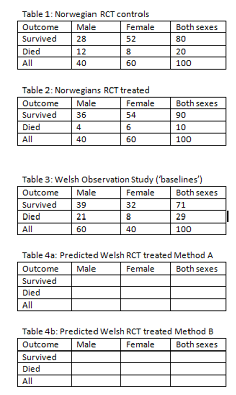
Hi again Suhail @s_doi. In order to clarify things with a fresh example, would you please apply Methods A and B to to predict the two possible results of a study in Wales (Tables 4a and 4b) from a baseline observational study in Wales (see Table 3) and the known result of a RCT in Norway (see Tables 1 and 2). This exercise was suggested by @AndersHuitfeldt during an explanation to me in post 540 Should one derive risk difference from the odds ratio? - #540 by HuwLlewelyn). Would you please show the results of applying Methods A and B by filling in the blank spaces in Tables 4a and 4b below.
1 Like
Hi Huw, only doing method A as using the RR (method B) is anybody’s guess and you can go with what you had previously calculated
All risks and odds are those for death
RCT
RLR males = 0.2593
RLR females = 0.7222
(Saturated model assuming this was a true product term and there was no random error induced artifact of the sample)
Observational study
Baseline risk Males = 21/60= 35% (odds = 0.5385)
Baseline risk females = 8/40 = 20% (odds 0.25)
Predicted risk males = 12.2% (converted from odds of 0.5385×0.2593)
Predicted risk females = 15.3% (converted from odds of 0.25×0.7222)
Addendum
I note that your post had marginal calculations so added method B here
Predicted risk males 11.6%
Predicted risk females 15%
Table in method B same as in method A
Note: These calculations assume no sample artifacts so both models are over-fitted. Had we removed the product term results would have been quite different. Also this highlights one safety net for users of method B - at low baseline risks we get numerically similar results explaining why an expected medical disaster through use of the RR over the last few decades has been averted
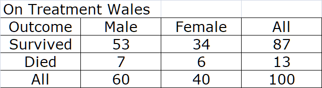
Thank you Suhail. So what you are saying is that in Method A you assume that the odds ratio is constant between the RCT in Norway and Wales and in Method B you assume that the risk ratio is constant between the RCT in Norway and Wales. This is what @sscogges suggested about a previous example if I recall correctly. You also tell us that at high risks the OR and RR are different but at very low risk the OR and RR become similar. All this is very well known of course. However if the baseline risk is high (e.g. 0.6) and the RR is 2, then the treated risk is 0.6 x 2 = 1.2 which is absurd. This is why @AndersHuitfeldt and others advocate using the switch RR in this situation to give 1-(1-0.6 x 1/2) to give 1- 0.2 = 0.8 instead of the silly 1.2. There is a lot more to the matter of effect measures of course such as associatively collapsible ORs, RRs and MRRs.
2 Likes
No, we can not assume any effect measure is constant as Sander has said many times and perhaps that is because I have been using the term “portability” instead of “variation independence” of the OR. I have now switched to this terminology. Both the RR and LR are variation dependent. However, the RR is one more step in the wrong direction in method B because of the added assumption that probabilities change linearly, which is inconsistent with Bayes’ theorem.
In this example and usually in low risk settings the numerical values and sometimes the numerical predictions come together, but as Frank aptly put it, the OR and RR measure different things and their numerical equivalence or difference gains significance only when interpreted wrongly.
Are you referring to one of my sentences in this quote?
Yes, the one above
Methods A & B are not based on constancy of these across populations but rather that these methods can be used to update probabilities based on evidence. Whether method A or B is the correct form of evidence is what is under discussion.
Huw, you are absolutely correct that Method A assumes the OR is the same in the population we have results for and in the population we’d like to generalize to and Method B assumes the same for the RR if we want these methods to actually be coherent. Not in the technical sense of coherency, just in the sense of actually having a chance at producing the correct answer. This is obvious from examining the equations behind the two methods.
From Suhail’s description of Method A
Convert r0 in new population to odds and multiply by ratio of RRs (i.e. odds ratio) obtained from study in original population:
\begin{align}
\frac{P(Y_1 | X_1 = 0)}{1 - P(Y_1 | X_1 = 0)} &\times \frac{P(Y_2 | X_2 = 1)/(1 - P(Y_2 | X_2 = 1)}{P(Y_2 | X_2 = 0)/(1 - P(Y_2 | X_2 = 0)} \\
& := \gamma
\end{align}
where the := symbol just indicates that we’re assigning the name \gamma to the quantity on the left-hand side.
The next step in the method is to treat \gamma as if it’s the odds for the outcome under treatment in the new population, and convert that to a probability to obtain P(Y_1 | X_1 = 1). But treating \gamma as if it’s the odds of the outcome under treatment in the new population only makes sense if we assume that the odds ratio is the same in the new population and the old population, since that’s what makes the relevant cancellations actually happen:
\begin{align}
&\gamma := \\
& \\
&\frac{P(Y_1 | X_1 = 0)}{1 - P(Y_1 | X_1 = 0)} \times \frac{P(Y_2 | X_2 = 1)/(1 - P(Y_2 | X_2 = 1)}{P(Y_2 | X_2 = 0)/(1 - P(Y_2 | X_2 = 0)} =\\
& \\
& \frac{P(Y_1 | X_1 = 0)}{1 - P(Y_1 | X_1 = 0)} \times \frac{P(Y_1 | X_1 = 1)/(1 - P(Y_1 | X_1 = 1)}{P(Y_1 | X_1 = 0)/(1 - P(Y_1 | X_1 = 0)} = \\
&\\
&\frac{P(Y_1 | X_1 = 1)}{1 - P(Y_1 | X_1 = 1)}
\end{align}
where the equality between lines 2 and 3 follows from assuming that the ORs are the same in the two populations. Without that assumption, \gamma is just some arbitrary quantity that has no guarantee of actually aligning with the odds of the outcome under treatment in the new population.
Similar calculations can be done for Method B to show how it assumes that the RRs are the same in the two populations.
Edit: Of course, which, if any, of these methods produces the correct answer will depend entirely on the reasonableness of those assumptions about the OR and RR.
1 Like