@AndersHuitfeldt has helped to transform my understanding of effect measure collapsibility. I understand that one purpose of collapsibility to epidemiologists is to be to try to use the marginal RRs or ORs of a RCT from those observed in one population (e.g. in Norway) to estimate what might be observed in a different population (e.g. in Wales) where the conditional risks based on a covariate (e.g. males / females) are different. However this can be done using the collapsible property of natural frequencies and natural odds, which I have known as long as I have been using ‘P Maps’ to be always collapsible (although I did not use that word). This is explained in my previous post ( Should one derive risk difference from the odds ratio? - #540 by HuwLlewelyn ). This illustrates the point about nomenclature made by @ESMD and perhaps the reason that it has taken me so long to understand @Sander and others.
What interests me as a clinician however, is how to apply the result of a RCT to patients with the same disease but various degrees of disease severity (fundamental to clinical practice) and also to apply them to patients with different baseline risks for other reasons (e.g. the presence of multiple covariates that change the baseline risks). This can be helped when conditional and marginal effect measures such as RRs and ORs are identical as well as being natural frequency and natural odds collapsible.
The RR and OR can be very helpful for low risks encountered in epidemiology (when they can be very similar numerically). However the RR not only gives implausibly large RDs at high probabilities encountered in the clinical setting familiar to me but also probabilities > 1 if the treatment increases risk (a problem that can be prevented by the switch RR of course). The OR does not have these bad habits and allows the marginal OR to be transported plausibly to baseline probabilities that are higher and lower than the marginal probability in a convenient way. However the OR is not an accurate model because when the marginal and conditional odds ratios are the same, p(Z=1|X=0) ≠ p(Z=1|X=0).
Another approach is to fit logistic regression functions independently to both the control and treatment data, but this too can provide biases (e.g. due to choice of the training odds used). My solution is to use any of the above when convenient for practical reasons and then to calibrate the results by regarding the ‘calculated curves’ as being provisional. I explained how I do this in another recent post: Risk based treatment and the validity of scales of effect , that also explores a different aspect of causal inference when dealing with multiple covariates.
Hi Huw, p(Y1|T)/p(Y1|C) and p(Y0|T)/p(Y0|C) are both RRs and LRs in the nomenclature of Bayes’ rule. In this direction they are LRs for Y as a test for T status.
In the other direction T as a test of Y status, you mixed up the nomenclature and this should be p(T|Y1)/p(T|Y0) and p(C|Y1)/p(C|Y0). These two are also LRs but this time are NOT RRs.
Note also that:
p(Y1|T)/p(Y1|C) divided by p(Y0|T)/p(Y0|C)
is exactly the same as:
p(T|Y1)/p(T|Y0) divided by p(C|Y1)/p(C|Y0)
That is why I can use either ratio of LRs interchangeably.
What you mean to say here is “…when the conditional odds ratios are the same, it does not equal the marginal odds ratio”. This is the definition of noncollapsibility and this whole discussion started because the causal inference group could not understand why this happens and called it an inaccuracy just as you did. What is the evidence that this is an inaccuracy? Just because we cannot get a weighted average of the conditionals to deliver the marginal does not imply inaccuracy and there needs to be a valid reason before noncollapsibility can be tagged “bad”
Also, averaging as you have indicated above is not interesting for decision making as Frank has said - please see Frank’s blog here
There is no “causal inference group” in this discussion. I speak as an individual, not as a member of some united front of causal inference researchers. Moreover, I understand “why this happens” (i.e. why the odds ratio is non-collapsible). I never called it an “inaccuracy”, can you please point out where you think this term was used?
The key question for discussion is whether we ever have reason for believing that an effect measure might be stable between different groups, and if so, whether we can pinpoint the applications in which such stability is expected to hold. Non-collapsibility is somewhat relevant, in part because I provided a proof that certain broad classes of data generating mechanisms will never lead to stability of a non-collapsible effect measure. But really, non-collapsibility is a red herring, since nobody even tried to formalize a biological generative model that leads to such stability. I don’t understand how collapsibility has taken on such an outsize role in this conversation.
The chance that conditional risks are different is lower than the near certainty that marginal effects are different, due to shifts from predominantly high-risk patients to predominantly low-risk patients or vice-versa. Still trying to wrap my head around the utility of marginal estimates.
This approach doesn’t use what we’ve learned about predictive modeling in the past 40 years. It should be contrasted with an additive (in the logit) model that properly penalizes all the interaction terms that are implied by the separate fitting approach, to avoid overfitting.
I am not at all experienced at fitting logistic regressions. I used the calibration method as a check. I expect that if the fitting was done with expertise using all the safeguards, the curves would be automatically well calibrated with no need for adjustment.
In a previous post I think that you said that when the marginal and both conditional RRs are the same (i.e. all three), this would be known as associational collapsibility. Do you think that this is the best term to use and are there synonyms in use too?
The distinction between “associational” and “causal/counterfactual” collapsibility is about whether the effect measures themselves are defined in terms of counterfactual or observed probabilities. The concept you are discussing is a different distinction. What you are referring to is called “strict” collapsibility. You can have “strict counterfactual collapsibility” and “strict assocational collapsibility”, thought “strict causal collapsibility” is a strange concept, because it always holds when you have no effect modification on a collapsible scale, and is better understood as just scale specific effect homogeneity.
Thank you. So if p(Y=1|Z=1) = 4/6, p(Y=1|Z=0) = 5/14 and (Y=1) = (4+5)/(6+14) = 9/20 would you think it reasonable to call this ‘strict natural frequency collapsibility’ (or some other term)?
I am not sure I understand you correctly here. If you shift from high risk to low risk patients, haven’t the conditional risks changed by definition?
A marginal estimate (on a collapsible scale) is useful because it is an average effect across a population. If I had to make a guess about what effect will apply in me, I could do worse than going with the average effect in the population that I am part of. Of course, I might prefer a more finely grained conditional estimate (i.e. an estimate representing the average effect in people who are more like me, in terms of some covariates believed to be relevant). But there is a significant tradeoff here in terms of statistical power, and unless my study is absolutely huge, I probably want to reserve my conditioning to only to the most significant effect modifiers.
Importantly, a marginal effect measure on a collapsible scale may in some sense be applicable to my estimate of my baseline risk regardless of what I choose to condition on to estimate my baseline risk. The conditional effect measure will be a better, more accurate estimate, but the marginal one is not a priori wrong.
In contrast, non-collapsible effect measures will only be applicable if I generate my baseline risk prediction using the exact covariates that were used in the model. If I generate my baseline risk predictions using some other covariates, I know mathematically that the conditional odds ratio is inapplicable.
Importantly: If you are using a minimal logistic model and getting “conditional” odds ratio estimates for the main exposure because the model includes main terms for the confounder (but no product terms), you get all these disadvantages and you aren’t even allowing the “effect” to differ between groups. This isn’t about conditioning to get an estimate that is more “personalized”, the estimate is the same for everyone, you have made it “conditional” in a way that reflects not variation in effects, only the mathematical peculariaties of your effect measure. Only when we start talking about product terms does it make sense to begin talking about the effect estimates becoming more personalized
Even when there is strict associational collapsibility of odds ratios (the marginal and both conditional RRs are exactly the same), the calculated prior probabilities of the findings Z=1 and Z=0 are different in the control and treatment population. It is as if p(Z=1|X=1) (from treatment) has changed due to the treatment to become different to the pre-treatment value of p(Z=1|X=0) (on control). This means that the odds ratio does not model the result of a RCT where the control and treatment populations are exchangeable and where p(Z=1|X=1) = p(Z=1|X=0). This suggests that a treatment curve calculated from the curve based control data should be regarded as provisional and ‘corrected’ by calibrating it.
I have looked at this example carefully using ‘P Maps’ and it appears that the answer to my previous question is as follows: p(Y1|C) = [3/20], p(Y1|T) = [10/20] and also P(Z1|Y1, C) = [2/3], P(Z1|Y0, C) = [8/17], P(Z1|Y1, T) = [4/10] and P(Z1|Y0, T) = [6/10].
When your are trying to predict an outcome Y=1 (e.g. death) conditional on control and a covariate Z=1, then the likelihood ratio P(Z1|Y1, C)/P(Z1|Y0, C) = (2/3)/(8/17) = 1.42. Therefore when you are trying to predict an outcome Y=1 (e.g. death) conditional on treatment and a covariate Z=1, then the likelihood ratio P(Z1|Y1, T)/P(Z1|Y0, T) = (4/10)/(6/10) = 0.67.
However, if you are trying to estimate the probability that a patient was on treatment when that patient had died, then as your say, the three RRs from the above become likelihood ratios. Thus p(Treatment|Death) = 10/13 = 0.77, p(Treatment|Death, Z=1) = 4/6 = 0.67 and p(Treatment|Death, Z=2) = 6/7 = 0.86.
This might be useful information when conducting a post-mortem and trying to work out the probability that the patient was on treatment or not when alive or inferring the cause of death. I would be interested to know how you would use this information to make clinical decisions when the patient was alive however!
Hi Huw, you are still mixing up the probabilities - can I suggest that you drop Z completely from the notation and if you refer to different strata just do that in the text…I will edit my post to remove Z as well so you can use the same probabilities. If yours do not match mine then what you are calculating is not comparable to what I am calculating.
Best to also post the 2 x 2 table with the calculations for clarity
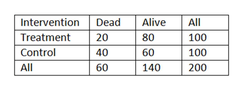
(Bayes rule (A) when T is evidence and D predicted and LR = p(T|A)/p(T|D)
p(D|T) = 1/(1+ p(A)/p(D) x p(T|A)/p(T|D)
20/100 = 1/(1+140/200)/(60/200) x (80/140)/(20/60) = 0.2
DIFFERENT Bayes rule (B) when D is evidence and T predicted and LR = p(D|C)/p(D|T) (and was RR in (A)
P(T|D) = 1/(1+ p(C)/p(T) x p(D|C)/p(D|T)
20/60 = 1/(1+(100/200)/(100/200) x (40/100)/(20/100) = 0.33
You are conflating (A) and (B) with your terms by mixing them up. Why are you estimating the probability of treatment conditional on death? This is the opposite of what we are trying to do.
Since I am using the ratio of the LRs ONLY it does not matter which direction it is calculated in as the ratio of LRs is direction independent and therefore the ratio of complementary RRs is always the ratio of LRs
As I have said previously and in my paper, LRs (and RRs) are only half the story as they update only unconditional probabilities. For example, if I want to update p(D) to p(D|T=1) then they are useful as in the diagnostic test setting.
In the study setting I want to update a conditional probability. Therefore I would like to update p(D|T=0) to p(D|T=1), now only the ratio of LRs (RLR) can be used and both ratios are the same so any can be used.
In your example, p(D|T=0) = 0.4 therefore odds = 0.67
0.67 × RLR = 0.67 × 0.375 = 0.25
p(D|T=1) = 0.25/1.25 = 0.2
Note that RLR is also a likelihood ratio but a different type of likelihood ratio when compared to the standard LR of Bayes’ theorem.
I can now update any baseline conditional probability using this RLR and these baseline conditional probabilities may differ across different populations but RLR is variation independent.
I’m not sure what you mean by “if you make assumptions about the data that lack an empirical framework”. I did not make any assumptions. I simply pointed out the assumptions that Method A and Method B are making in your example.
Regarding your addendum, I’m fairly sure that I have grasped the point. You have a dataset representing data from a clinical trial conducted in a population (Stratum 2). You have another population (Stratum 1 in the example), and you would like to predict the probability of the outcome given the treatment in this population knowing only the baseline risk in Stratum 1 and the results of the trial conducted in Stratum 2. You outlined two methods for doing so, Method A and Method B, which give different results. You believe the discrepancy is due to Method B violating Bayes’ theorem, and that Method A is to be preferred because it respects Bayes’ theorem (please correct me if I’m wrong here). As I and others have pointed out, your claims about methods violating Bayes’ theorem are not coherent, and the source of the discrepancy actual lies in the different assumptions each method makes about which effect measures are constant across strata.
You also seem to think that there must be (or should be) a way to decide which method to use based purely on observed quantities available in the data. To show you why this is generally not possible, let’s consider data from another trial conducted in another population (we’ll call it Stratum 3):
Y=0
Y=1
X = 0
70
30
X = 1
55
45
For simplicity, we ignore the issue of sampling variability and assume that the probabilities implied by these counts are estimated with extremely high precision. Now suppose, as in your example, we want to predict the probability of the outcome (Y = 1) under treatment (X = 1) in another population (let’s call it Stratum 4) using only the results from the trial in Stratum 3 and the knowledge that the baseline risk in Stratum 4 is equal to 0.1. Applying Method A, we
get a predicted probability of 0.175. Applying Method B, we get a predicted probability of 0.15 (please double check my calculations). So, which is correct? Well, suppose that God comes down and reveals that given the full population of Stratum 4, the distribution would look like
Y = 0
Y = 1
X = 0
0.90
0.10
X = 1
0.85
0.15
So Method B (which you claim violates Bayes’ theorem) gives us the correct answer of 0.15 while Method A gives us an incorrect answer of 0.175.
We now have two examples, one where Method A provides the correct answer and one where Method B provides the correct answer. In both cases, the method that gave the correct answer was the one that made the correct assumption about which effect measure was constant across strata (the OR in the first example and the RR in my second example). Hopefully this demonstrates why trying to come up with a way to decide which method to use based solely on the available data is not in general possible.
Question for discussion: Is anyone other than me getting concerned yet about the fact that BMJ Evidence-Based Medicine published a paper by Suhail ([Likelihood ratio interpretation of the relative risk | BMJ Evidence-Based Medicine ]) in which the highlighted key message is that “The interpretation of the risk ratio as an effect measure in a clinical trial is naïve and better replaced by its interpretation as a likelihood ratio” because of this alleged “conflict with Bayes theorem”?
Yes, I am concerned for a very practical reason. As an applied statistician, I’m tasked with responding to stats-related reviewer comments on papers and grant applications. I would be very annoyed if I did a RR-focused analysis and got a comment from a reviewer citing this paper to tell me that I had violated Bayes’ theorem.