Suppose that the effect of an intervention versus control on an outcome (denoted ‘Y’) in a randomized trial will be assessed in an unadjusted fashion, e.g., using a t-test. We know that the operating characteristics of this test, namely the specified type-I error probability, does not depend on the distribution of covariates (denoted ‘X’) that are simultaneously measured. Thus, the observed balance or imbalance of sampled covariates should not impact the interpretation of the test results. However, there is anecdotal evidence that this is commonly misunderstood, and that readers sometimes discount the findings of a study due to perceived covariate imbalance. To avoid this, the argument is that covariate imbalance information should simply be omitted from publications that describe the main results of such randomized trials.
What if the reported P value at each of the covariates was instead that of:
anova(full.model.minus.covariate, full.model)
Where:
full.model <- glm(treatment.group ~ age + sex + ... + covariateZ)If you fail to adjust for pre-specified covariates, the statistical model’s residuals get larger. Not good for power, but incorporates the uncertainties needed for any possible random baseline imbalances.
Table 1 for a randomized clinical trial traditionally contains baseline variables as rows and treatment group as columns, with an additional column for “All Treatments”. Sometimes p-values are added, as in the recent guidelines from NEJM. The latter practice is clearly misguided, because p-values are inferential quantities, and the inference is for the population from which the sample came. Suppose that one tested whether the mean age is the same in treatments A and B. The population inference would involve randomizing half of all people to A and half to B at random. But their mean age would be identical in this population, so the null hypothesis is already known to be true. Hence the p-value can have no meaning in this context.
Then the question becomes “should we stratify by treatment in Table 1”? I submit that the mere act of stratifying by treatment is at odds with how randomization works. The only reason to stratify is to compare the summary statistics by treatment. Any differences in summary statistics are by definition due to chance. So here is a list of reasons to only present the “All Treatments” column in Table 1:
- There is a significant psychological problem. A reader who does not like the treatment, endpoint, study design, or authors will seize an apparent imbalance in baseline characteristics to criticize the accuracy of the study’s treatment comparison result.
- All imbalances are by definition due to chance, and we expect imbalances to always be present to some degree.
- Related to the previous item, if you generated a “phantom Table 1” with the same number of rows as the real Table 1, and every variable created using a random number generator, you’ll see the same extent of imbalances.
- The set of baseline characteristics included in Table 1 is somewhat arbitrary, so looking for apparent imbalances is somewhat arbitrary.
- If there is an imbalance in favor of treatment A, one can always find another imbalance that is equally in favor of treatment B if sufficiently many additional baseline characteristics are examined. Thus the imbalances cancel anyway.
- Researchers who think that a particular baseline covariate imbalance might explain away a treatment benefit do not even take the time to compute whether the magnitude of the imbalance is sufficient to explain the magnitude of the treatment difference. And if one were to compute an uncertainty interval for the fraction of the treatment effect that could possibly be explained by an apparent covariate imbalance, she would be surprised at the width of this uncertainty interval.
- How often do researchers look for covariate imbalances that might explain away a non-difference between treatments?
- Most importantly, as Stephen Senn describes here and here, the unadjusted statistical test for comparing A and B is completely valid in the face of apparent treatment imbalances. The A-B comparison is just as valid when the researchers do not even measure any baseline covariates so there are no covariates even available for Table 1.
To expand on the all-important last point, there are two clear reasons that the pre-specified statistical test, whether adjusted for pre-specified covariates or not adjusted for any covariates, remains valid in the face of observed imbalances.
- Statistical inference is based on probability distributions. To know these distributions it is necessary to know the probability distribution of variables, not their observed values. So it is sufficient to know that the tendency was for baseline covariates to be balanced. It’s the tendency that goes into inference.
- The p-value is the probability of another dataset being more extreme than the current data if H0 is true. The type I error is the probability of making an assertion of efficacy when in fact there is no efficacy or harm of the treatment. The chance of falsely attributing observed treatment differences to something other than treatment is present in both p and type I error. We needlessly partition all the possible reasons for a false observed treatment effect into covariates and other unknown causes including complete randomness. The statistical test for A:B does not know anything about such partitioning of reasons for the observed effect.
Simulation
To get a sense of how easy it is to find counterbalancing covariates once a covariate with a positive imbalance (which we’ll take as an imbalance in the direction of explaining away the apparent treatment difference) is found, consider 1000 repetitions of a trial with 100 subjects and with 10 n(0,1) continuous covariates. A positive imbalance is taken as a covariate with the difference in means of the covariate between treatments that is > 0.3. This happened in about 1/2 of the 1000 trials. Consider the subset of the simulated trials with exactly one positive imbalance. Some of these trials will have an additional positive imbalance before a negative imbalance (counterbalance). Of those trials for which the first negative imbalance is not preceeded by a + imbalance in the new covariates, we find that if one measured 40 additional covariates, one always finds a counterbalancing factor. The average number of additional covariates that need to be examined for this to happen was 7.
n <- 100
k <- 10
nsim <- 1000
set.seed(1)
ne <- jc <- integer(nsim)
nc <- 0
for(i in 1 : nsim) {
  ## Simulate a difference in two means with data SD of 1.0
  x <- rnorm(k, sd=sqrt(4 / n))
  ne[i] <- sum(x > 0.3)
  if(ne[i] == 1) {
    ## Simulate 200 additional covariates (never needed > 40)
    x  <- rnorm(200, s=sqrt(4 / n))
    ## Find first counterbalance not preceeded by another imbalance
    ## in the original direction
    j <- min(which(x < -0.3))
    if(j == 1 || max(x[1 : (j - 1)]) < 0.3) {
      nc <- nc + 1
      jc[nc] <- j
    }
  }
}
jc <- jc[1 : nc]
## Distribution of number of positively imbalanced covariates in first 20
table(ne)
ne
  0   1   2   3   4   5
487 359 129  23   1   1

## Distribution of # additional covariates that had to be examined to
## find a counterbalance without being preceeded by another + imbalance
table(jc)
jc
 1  2  3  4  5  6  7  8  9 10 11 12 13 14 15 16 17 18 20 25 28 29 40
26 22 17 15 10 22 10 11  6  5  8  8  5  3  4  5  4  1  1  1  1  1  1

w <- c('Number of trials with exactly one + imbalance:', sum(ne == 1), '\n',
       'Number of such trials with a - imbalance in additional covariates not\n preceeded by another + imbalance:', nc, '\n',
       'Average number of additional variables examined to find this:',
       round(mean(jc)), '\n')
cat(w, sep='')

Number of trials with exactly one + imbalance:359
Number of such trials with a - imbalance in additional covariates not
 preceeded by another + imbalance:187
Average number of additional variables examined to find this:7
Proposed Replacement for Table 1
Any space used in a published paper needs to be justified. I submit that the overarching principles that any display in a clinical trial report must follow are
- The information be unique
- The information provides insight
Table 1 is the opportunity to describe to the reader who got into the trial. It can also provide the opportunity to provide exceptionally richer information that is usually seen by the reader: who suffered the main trial endpoint? With this and the above two criteria in mind, here is a modest proposal for a replacement for Table 1: show graphically the baseline distributions (all subjects combined) along with the relationship between that baseline variable and the outcome. In the example below, the SUPPORT study is used. For this example, only continuous or semi-continuous baseline variables are included. The outcome variable is death within hospital and each y-axis is the estimated probability of hospital death. Day 3 of hospitalization is the baseline period. R code used to create this graph appears after the graph.
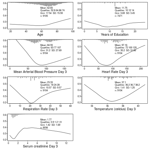
require(Hmisc)
getHdata(support2)
d <- support2[Cs(age, edu, meanbp, hrt, resp, temp, crea, hospdead)]
png('table1.png')
spar(mfrow=c(4, 2), left=-3)
g <- function(x) round(x, 2)
for(i in 1 : 7) {
  z <- d[[i]]
  x <- z[! is.na(z)]
  xl <- range(x)
  plsmo(z, d$hospdead, datadensity=FALSE, xlab=label(x),
        ylim=c(.2, .6), ylab='')
  histSpike(x, add=TRUE, frac=0.15, side=3)
  w <- paste0('Mean: ', g(mean(x)), '\nQuartiles: ',
              paste(g(quantile(x, (1:3)/4)), collapse=' '),
              '\nGini: ', g(GiniMd(x)),
              '  SD: ', g(sd(x)),
              '\nn: ', length(x))
  m <- mean(par('usr')[1:2])
  y <- 0.5
  for(j in 1:4) {
    y <- y - 0.038
    text(m, y, w[j], adj=0, cex=.8)
  }
  }
dev.off()
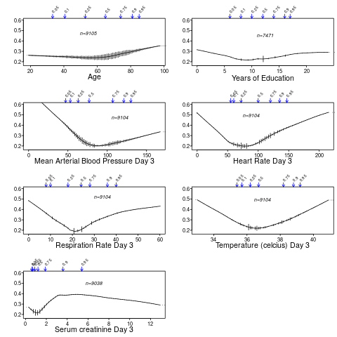
You can also use the higher-level R Hmisc package function summaryRc:
png('table1b.png')
spar(mfrow=c(4,2), top=2, left=-2)
summaryRc(hospdead ~ age + edu + meanbp + hrt + resp + temp + crea,
          data=d, ylab='', ylim=c(.18,.6), datadensity=TRUE,
          srt.quant=45, scat1d.opts=list(frac=.05))
dev.off()
Further Reading
- Out of Balance by Darren Dahly
- Does the “Table 1 fallacy” apply if it is Table S1 instead? by Dean Eckles
This is similar to what @f2harrell suggests below, except that he suggests presenting unadjusted associations in a graphical manner, whereas you are suggesting to summarize the adjusted association using a p-value. Either approach seems reasonable to me, although the former presents more, and simpler information.
I prefer adjusted estimates against the outcome. But he was proposing a test of global covariate balance. Though better than individual tests it’s still not appropriate because the study was randomized.
This would be a huge improvement on the current way papers are presented. But the only way to convince journals is for it come from a weighty consortium of statisticians
Trialists should endeavor to inspect the quality of their randomization.
Why? Two seemingly identical trials can lead to conflicting results if a very important covariate is stratified in one trial and imbalanced in the other AND that covariate is an effect modifier.
My complaint about current practice:
-
I agree that presenting a “table one” devotes far too much time and too much attention to the relevance of balance. In the paper, the statistician should just say, “Randomization was inspected.”
-
I think better effort must be made to describe and measure prognostic factors that could be confounders when deploying the treatment in a non-participant population.
-
A better way to inspect randomization than doing billions of T-tests for frequency differences by treatment assignment is to actually redo the main analysis using some form of adjustment or weighting. Theoretically, they should have no impact and it reduces the inference down to a single comparison rather than many.
Well, I am convinced! Thank you for the really clearly articulated explanation. Not sure there can be a counter argument for keeping stratified table 1’s in response to this. I really like the proposed summary presentation of baseline covariates with outcome to provide richer information but may not be ready to get rid of a table 1 in its recognisable form with pooled data yet describing the participants.This suggestion could be used for a new table 2 or later?
I’m entirely on board with these suggestions.
What’s your favorite citation for justifying this approach when you (inevitably) get reviewer comments asking for a Table 1 stratified by treatment allocation and filled with P-values?
Fun question! It is an inevitable request but less so from journals in my experience and more often from investigators. I have in the past used an early Altman paper and a paper by Senn. I used to work in Dougs unit and came from the approach not to test, but its ok to look- now convinced by your philosophical argument not too look. Next interesting challenge will be to start proposing this recommendation. A published article needed- anything written yet on this?
The point about effect modification is important. But it’s not that ignoring this is completely wrong; more so it’s that the treatment effect will be a kind of average over levels of the interacting factor, so will not apply well to individuals even though it’s right “on the average”.
To say “randomization was inspected” is not specific enough. The randomization process should be inspected and mentioned. Not covariate balance, which just reflects random occurrences.
Instead of “describe and measure prognostic factors” I’d say “pre-specify the most important prognostic factors” and adjust for them come hell or high water. This also does away with the need for your 3.
There are 4 references in Section 13.1 of BBR.
I agree with this. When Adam first suggested it I got the feeling that “randomization inspected” is too vague and is moving away from being more open, which I feel is counter to what a lot of people in research are trying to do.
I find the arguments here very convincing. I’ve been thinking about using graphical dsiplays for “Table 1” too and this seems a much better way to communicate the important information than tedious and hard to interpret tables. I guess the question is really: what is this table(or collection of graphs) for? I would agree with Frank that it’s primarily about describing the population in the trial; I suspect most people would say that it’s about assessing balance and the success of randomisation - which is crazy really because we are almost always sure that our randomisation processes are sound, and most of the variables in “Table1” don’t play any role in randomisation, so it’s probably unrealistic to expect them to show up any problems.
The NEJM justification for using p-values in Table 1 was to detect problems in randomisation or possible malpractice (https://simongates.com/2018/08/29/nejm-definitely-the-last-time/) which sounds a bit of a stretch to me.
A very interesting discussion! Particularly if we are analyzing these data using frequentist methods, I come down on the side of pre-specifying known important prognostic factors and planning to adjust for them irrespective of any imbalances that may or may not arise in the data circumstantially.
My reasoning is as follows: In a frequentist world, we need to ask ourselves to think about a hypothetical scenario under which the study at hand were repeated infinitely many times under identical circumstances. If one’s decision–through inferential, graphical, or descriptive summary measures–to place a prognostic variable into a model is based on imbalances (perceived or real) in the observed data, he or she has obfuscated his or her standard errors. Confidence intervals from the model will not have valid coverage. What’s more, if you are modeling a parameter using a non-collapsible link function, the parameter you target is not invariant across study replicates–namely, you change it each time you make a different decision about which variables to adjust for.
If a particular prognostic factor is not balanced across treatments, we know that this is due to random chance by virtue of the randomized nature of treatment. Under a frequentist framework, that same variable would show a comparable amount of imbalance in the opposite direction in some other theoretical study replicate almost surely. Strictly speaking, then, any observed imbalance in any factor (prognostic or otherwise) across treatment levels does not induce a bias if left unadjusted for. Rather, imbalances in any covariates are one (of several) factors that explain the overall variability of the estimate.
Finally, adjustment for known prognostic factors is understood in many settings to increase power, and so doing this (i.e., planning to do this) is unlikely to hurt you.
This is a very nice angle, getting at the fundamental meaning of sampling distributions when using frequentist inference. I read you as saying that if one looks for observed imbalances, and does anything about it, the sampling distribution is ill-defined because there will be by definition different covariates imbalanced at each study replication, and positive imbalances can even turn into negative ones.
Hi @SpiekerStats, thanks for sharing this additions lens on the issue. If I understand this correctly, it seems that a similar problem (described in the quoted text) might occur if the model were modified in some other way, e.g., by modifying the link function or considering a transformation of the response, or by modifying the error structure. If so, how do we reconcile this with our use of model diagnostics in this context?
I agree with this conclusion–particularly if these choices are tied to the data and if different hypothetical study replicates would potentially cause you to make different choices. It’s really such a tough thing, because this problem seemingly demands not just that you get the model right, but that you get it right the first time without ever using your data to guide you.
To the extent possible, I try to rely on a pre-specified semi-parametric regression methods, together with splines. That one can consistently estimate the coefficient(s) corresponding to treatment effects even if the splines for the prognostic variables are not correctly specified is a huge help. An a priori choice to employ Huber-White errors would further prevent me from worrying unduly about a mis-specified error structure. If I really want to estimate a difference in means, it’s going to be very hard to convince me to change the link function away from the identity or to transform the outcome post-hoc, not just because I’m changing a model, but because I’m changing the question at hand. I hope these choices help justify my personal tendency (preference?) not to give model diagnostics a great deal of consideration for most of the association studies I work on.
But then, once we’re in a world where we need to start relying on random draws from a predictive distribution (e.g., in parametric g-computation), this gets so much more dicey, and the problem of what to do when confronted with evidence of an incorrect model really comes to life. Absent nonparametric alternatives, the simplest potential remedy I can think of is to use a training set for model building and learning–and then using the trained model structure on the remainder of the data to obtain the quantitative evidence about the parameter at hand and, in turn, to derive conclusions. There are obvious shortcomings–not the least of which is the presumption of enough data to justify the power cost  .
.
A lot of food for thought. For non-statistician readers, the link function is a very important part of the model. In the logistic model the link is the logit (log odds) function \log(\frac{p}{1-p}) and in the Cox proportional hazards model it is log hazard or equivalently log-log survival probability. In ordinary regression the link function is the identify function, e.g., we model mean blood pressure directly from a linear combination of (possibly transformed) covariates.
When there is no uncertainty about the link function, the Bayesian approach has some simple ways to handle uncertainty about the model. For example, if one were unsure about whether treatment interacts with age, an interaction term that is “half in” the model could be specified with Bayes by putting a skeptical prior distribution on the interaction. This logic also applies to accounting for a list of covariates that you hope are not that relevant, by penalizing (shrinking) the effects of these secondary covariates using skeptical priors.
When the link function itself is in question, you can essentially have a Bayesian model that is a mixture of two models and let the data “vote” on these. For example you could have a logit and a log-log link. The resulting analysis would not give you the simple interpretation we often seek, e.g., a simple odds ratio for treatment. Odds ratios and all other effect measures would be a function of the covariates. But one could easily estimate covariate-specific odds ratios and covariate-specific absolute risk differences in this flexible setup.
The key is pre-specification of the model structure. In the frequentist world we must specify the complete list of covariates to adjust for before examining any relationships between X, treatment, and Y. With Bayes we can pre-specify a much more complex model that includes more departures from basic model assumptions. As n \rightarrow \infty, this will reduce to the simple model should that model actually fit, or it will automatically invoke all the model ‘customizations’ including not borrowing much information from males to estimate the treatment effect for females should a sex \times treatment interaction be important. For smaller n, such a Bayesian model would discount the interaction term which results in borrowing of information across sexes to estimate the treatment effect. To take advantage of the Bayesian approach one must pre-specify the general structure and the prior distributions of all the parameters that are entertained. That’s where clinical knowledge is essential, e.g., how likely is it apriori that the treatment effect for males is more than a multiple of 2 of the treatment effect for females?
Doesn’t fitting the conditional model change your the meaning of your parameter because inference is conditional on the other covariates in the model? I.e. E(Y|T=1, AGE=30) - E(Y|T=0, AGE=30) is not equal to E(Y|T=1) - E(Y|T=0), except with identity link. But, it seems the goal of the clinical trial is to estimate E(Y|T=1) - E(Y|T=0) (or E(Y|T=1)/E(Y|T=0) ). I think @SpiekerStats you are right that you need to fit the correct mean model to get probably smaller and lower variance standard error estimates (even if using robust SE estimates), but I think the target parameter should still be the same E(Y|T=1) - E(Y|T=0), instead of interpreting the parameter for treatment from the logisitic regression model.