Some thoughts on uniform prior probabilities when estimating P values and confidence intervals

[EvZ]

It would be nice if you found our discussion illuminating, but I think you’re just being sarcastic. I certainly had a very poor experience trying to discuss your preprint with you.

In a statistics paper, we try to be very clear about the model and the statements we derive from it. In particular, we try to be very clear about how all the variables are defined.

Your preprint is quite different from a statistics paper. It has some figures, some numbers and a lot of talk (“all possible observed means of a continuous variable are conditional on the universal set of all numbers” and things like that). There are no clearly defined variables, there is no clearly defined model and there are no clearly derived statements.

Of course, the fact that your preprint doesn’t look like a statistics paper does not mean there’s anything wrong with it! So I wanted to be helpful by introducing proper notation to clarify your model and your conclusions. This turned out to be extremely difficult. Finally, in post 215 (!) we managed to agree on

Model: We are assuming the uniform distribution on \beta and
b \mid \beta,v_1 \sim N(\beta,v_1) \quad \text{and}\quad b_\text{repl} \mid \beta,v_2 \sim N(\beta,v_2).
Moreover, b and b_\text{repl} are conditionally independent given \beta.

Now that we have a well-specified model, we can do math. If we define z_\text{repl} = b_\text{repl}/\sqrt{v_2}, then we have the (provably) correct statement

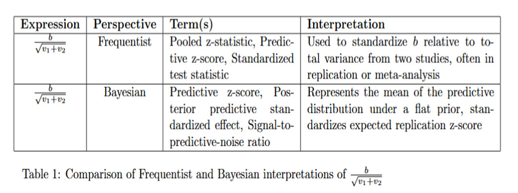
P(z_\text{repl} > 1.96 \mid b,v_1,v_2) = \Phi\left( \frac{b - 1.96\sqrt{v_2}}{\sqrt{v_1+v_2}} \right)

and the (provably) false statement

P(z_\text{repl} > 1.96 \mid b,v_1,v_2) = \Phi\left( \frac{b}{\sqrt{v_1+v_2}} - 1.96\right).

I was amazed that you continued to argue in favor of the false statement. That’s just crazy! The issue was finally resolved by introducing a new variable, namely z^\text{Huw}_\text{repl} =b_\text{repl} /{\sqrt{v_1+v_2}}. Now we have the true statement

P(z^\text{Huw}_\text{repl} > 1.96 \mid b,v_1,v_2) = \Phi\left( \frac{b}{\sqrt{v_1+v_2}} - 1.96\right).

I was again amazed that you claimed I misrepresented your views when I had derived your own “predictive replication probability” in the context of the model we had agreed on! Maybe you didn’t like the name z^\text{Huw}_\text{repl}. Perhaps I should have used x_\text{repl}=b_\text{repl} /{\sqrt{v_1+v_2}}. A rose by any other name …

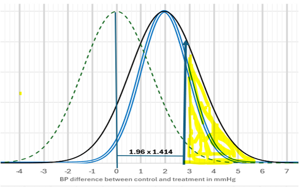
Now that we have some true statements, we can discuss the merits of your contribution. Assuming the uniform prior on \beta, you compute the predictive probability of the event |z^\text{Huw}_\text{repl}| > 1.96. I do not think this is useful for two reasons

1. The uniform prior on \beta is unrealistic.
2. The event |z^\text{Huw}_\text{repl}| > 1.96 is uninteresting because “replication success” is commonly defined as |z_\text{repl}| > 1.96.

In closing: The main problem I’ve had trying to communicate with you about math and statistics, is that you seem to think in terms of “my” and “your” statements. However, in a correctly specified model there are only true and false statements, and we can use math to sort out which is which. Once we have a true statement, we can discuss its merit or usefulness.

[HuwLlewelyn]

@EvZ

It would be nice if you found our discussion illuminating, but I think you’re just being sarcastic

This post was deleted in error. I have just found out how to restore it and deleted the duplicate!

I found our discussion illuminating because it revealed a different approach to mathematical modelling from mine (which is to use mathematical models to provide a numerical version of a scientific hypothesis to be tested). It also reminded me of the problems with statistical terminology when trying to explain something, perhaps because of the differences between Frequentist and Bayesian concepts and terminology. For example, I managed find Table 1 below on the internet. What terms do you think that I should use for b/\sqrt{v_1 + v_2}?

[EvZ]

For example, I managed find Table 1 below on the internet.

Are you kidding me? Who knows what some random table from the internet means if you don’t even provide the context. The fact that they use the same symbols doesn’t mean they have the same meaning as for us.

Anyway, I’m really done with this. It’s clear to me what you’re trying to do and I don’t think it’s useful for anything. On the other hand, you don’t want to give up on fantasizing how your unique aproach to modelling has uncovered the reason for the “unexplained” replication crisis. You conveniently ignore that your “modelling” (1) doesn’t involve any data, (2) is based on the uniform prior on \beta which is unrealistic and (3) is aimed at a criterion for “replication success” that nobody uses.

[HuwLlewelyn]

@EvZ

You conveniently ignore that your “modelling” (1) doesn’t involve any data, (2) is based on the uniform prior on \beta which is unrealistic and (3) is aimed at a criterion for “replication success” that nobody uses.

I cannot allow you to make assertions that are clearly untrue.

(1) I do use data. I have tested the HL model against your data and that of the Open Science Collaboration data and they align closely.

(2) You assert that uniform prior on \beta is unrealistic but I am merely assuming it for the purpose of testing it as part of a hypothesis

(3) The criterion for replication success in the HL model is the probability of getting P≤0.05 again (or p(Z_repln > 1.96 again), which is what the Open Science Collaboration and others use. It is therefore incorrect to say that “nobody” uses it.

I am not 'fantasizing" but testing a hypothesis. Please!

[EvZ]

(1) As we agreed, your model is

Model: We are assuming the uniform distribution on \beta and
b \mid \beta,v_1 \sim N(\beta,v_1) \quad \text{and}\quad b_\text{repl} \mid \beta,v_2 \sim N(\beta,v_2).
Moreover, b and b_\text{repl} are conditionally independent given \beta.

Now tell me, which part of this completely generic model (which is also the basis in Goodman, 1992) was informed by data?

(2) I know the uniform prior does not align with reality because I’ve studied it. For example, you can have a look at Figure 1 in my paper with Goodman.

(3) The (in)famous result of the OSF paper is (I quote):

Ninety-seven percent of original studies had significant results (P < .05). Thirty-six percent of replications had significant results;

In our notation, this means that 97% of the original studies had |b/\sqrt{v_1}|>1.96 while 36% of the replication studies had |b_\text{repl}/\sqrt{v_2}|>1.96. It does not mean that 36% of the replication studies had |b_\text{repl}/\sqrt{v_1+v_2}|>1.96.

[HuwLlewelyn]

@EvZ

The (in)famous result of the OSF paper is (I quote):

Ninety-seven percent of original studies had significant results (P < .05). Thirty-six percent of replications had significant results;

In our notation, this means that 97% of the original studies had |b/\sqrt{v_1}|>1.96 while 36% of the replication studies had |b_\text{repl}/\sqrt{v_2}|>1.96. It does not mean that 36% of the replication studies had |b_\text{repl}/\sqrt{v_1+v_2}|>1.96.

My analysis of the Open Science Collaboration (OSC) data is summarised in the bottom line of the Table 2 below, which is an image of my Excel spreadsheet. As you can see, the HL expression predicts 34.2% replication rate based on the mean P-value in that paper of 0.028 (near to the replication rate for the P=0.03 from the Cochrane data in your paper with Goodman in 2022). However, this assumes that n2 = n1 but we know from the OSC paper that the power was higher at 92% on average in the second replicating studies. If we assume that it was 80% on average in the first studies, then the replication rate when n2 is larger in keeping with a power of 92% on average becomes 36.2% according to the HL expression, which corresponds exactly with what was discovered in the paper (i.e. 36.1%). I don’t think you can keep claiming that all this is a co-incidence.

Table 2

[EvZ]

You know about apples and oranges? That they’re not the same?

Your formula is predicting the frequency of the event |b_\text{repl}/\sqrt{v_1+v_2}| > 1.96 and you are comparing it with the frequency of the event |b_\text{repl}/\sqrt{v_2}| > 1.96.

This confusion happens because you insist on referring to both b_\text{repl}/\sqrt{v_1+v_2} and b_\text{repl}/\sqrt{v_2} as “the” z-statistic.

This is such a basic mistake. And you keep making it over and over and over and over again. Maddening!

[HuwLlewelyn]

@EvZ

This confusion happens because you insist on referring to both b_\text{repl}/\sqrt{v_1+v_2} and b_\text{repl}/\sqrt{v_2} as “the” z-statistic.

Why don’t we call them the Replication Test Statistic?

[EvZ]

For better of worse, “replication success” is commonly defined as b_\text{repl}/\sqrt{v_2} > 1.96. That’s how the authors from the OSF paper define it, and that’s how Goodman and I define it in our paper from 2022.

So, you should refer to b_\text{repl}/\sqrt{v_2} as the replication z-statistic, and to b_\text{repl}/\sqrt{v_1+v_2} as “just some useless statistic nobody is interested in”.

I know you will ignore this advice as you have ignored everything I tried to explain in the past 3 weeks. It’s clear that you much prefer to do your Excel calculations and imagine how that validates your generic little model.

I’m doing what I should have done 3 weeks ago; signing off!

[f2harrell]

Editorial comment: @HuwLlewelyn it is time to move past considering a statistic that has a variance term from the first study as a “replication statistic”.

[HuwLlewelyn]

Thank you. OK. Using the above terminology:

When z_1 is the original z statistic from which we calculate the original study’s P value, then z_1 = \dfrac{b}{\frac{s}{\sqrt{n_1}}} = \dfrac{b \sqrt{n_1}}{s}

and when {s}{\sqrt{n_2}} is the standard error of z_2 (the replication z statistic with unknown b_{repl}),

Then by substituting the above in the following and rearranging

P(z_{repl}>1.96∣b,s, n_1, n_2) = Φ(\dfrac{b}{\sqrt{ \left( \frac{s}{\sqrt{n_1}} \right)^2 + \left( \frac{s}{\sqrt{n_2}} \right)^2 }}-1.96)

we get

P(z_{repl}>1.96∣b,s, n_1, n_2) = Φ(\dfrac{b}{\frac{s}{\sqrt{n_1}} \cdot \sqrt{1 + \frac{n_1}{n_2}}}-1.96)

When n_1 = n_2 we get

P(z_{repl}>1.96∣b,s, n_1, n_2) = Φ(\dfrac{b}{\frac{s}{\sqrt{n_1}} \cdot \sqrt{2}}-1.96)

But when P is the one-sided P value for the original study,

b/\left( \frac{s}{\sqrt{n_1}} \right) = \Phi^{-1}(P)

Therefore by substituting the above, we get:

P(z_{repl}>1.96∣b,s, n_1, n_2) = Φ(\Phi^{-1}(P) {/ \sqrt{2}}-1.96)

This means that when n_1 = n_2 we can estimate the probability of replication directly from the P_-value without knowing b, s, n_1 or n_2:

P(z_{repl}>1.96∣Pvalue) = Φ(\Phi^{-1}(P) {/ \sqrt{2}}-1.96)

This is how the probabilities of replication were calculated in Tables 1 and 2 of my previous posts.

[EvZ]

@HuwLlewelyn

By substituting the above in the following and rearranging

P(z_{repl}>1.96∣b,s, n_1 n_2) = Φ(\dfrac{b}{\sqrt{ \left( \frac{s}{\sqrt{n_1}} \right)^2 + \left( \frac{s}{\sqrt{n_2}} \right)^2 }}-1.96)

Still the exact same mistake. Absolutely hopeless.

PS You’re also introducing a new mistake by calling both estimates “b”.

[HuwLlewelyn]

@EvZ

Still the exact same mistake. Absolutely hopeless.

PS You’re also introducing a new mistake by calling both estimates “$b$”.

If I am making a mistake, please explain why that my probabilities predict the frequencies of replication accurately in my previous Table 2 but your calculations do not do so. I show in today’s post why the result of my calculations are not coincidence. The first expression in today’s post is simply based on the traditional way of getting a pooled estimate of z when comparing the distributions of data from two limbs of a RCT.

[EvZ]

It’s a math mistake which I’ve explained many times now. It simply does not follow from “substituting and rearranging” as you claim. I’m not going to respond to this nonsense anymore.

[HuwLlewelyn]

@EvZ

PS You’re also introducing a new mistake by calling both estimates "b".

You keep saying that I am making mistakes, which I take seriously but can never understand what you mean because you have not been specific. leaving me to keep guessing. (There is an old joke about “How do you keep a fool guessing?”. The answer is “I’ll tell you later!”)

Is b_{repl} in your expressions a point value and if so how do you estimate it in order that you can evaluate z_2 = \dfrac{b_{repl}}{\frac{s}{\sqrt{n_2}}} = \dfrac{b_{repl} \sqrt{n_2}}{s}? I do not attempt to make a point estimate of b_{repl} because I don’t try to guess what it is; I only estimate its distribution conditional on the observed b and a flat prior. This is why I use b in my expressions including the one formed by ‘rearranging’, which I had hoped that you would like. Is the fact that I only consider the distribution of b_{repl} that is the fundamental difference between our approaches, which you consider to be a mistake on my part? This is one opinion that I have heard about the difference between our models. If you do not wish to reply, don’t worry. Maybe someone else can help.

[R_cubed]

@HuwLlewelyn

You keep saying that I am making mistakes, which I take seriously but can never understand what you mean because you have not been specific

1. Formally, your notation b implies the estimates b1 and b2 are equal in fact, not merely equal in expectation. You should rewrite that as b_1 and b_2 where the understanding is they are not.
2. A general formula for weighting standardized Z scores is \frac{\Sigma w_1Z_1 ... w_nZ_n} {\sqrt{\Sigma w_1... w_n}} The fact you are subtracting 2 z scores makes no difference, so long as you do the weighting properly, your result will also be a Z score wtih a distribution of N(0,1) under the null hypothesis. None of your attempts at mathematics acknowledges this.

[HuwLlewelyn]

@R_cubed

Formally, your notation b implies the estimates b1 and b2 are equal in fact,

Thank you for your comment.

Please understand that although I have a 'b' for z1, I don’t have a b_{repl} for z2 (only the SE for the distribution of z2). I have a SE only for z2 in my expression and a combined SE from v1 and v2. So therefore weighting according to b and a point estimate of an absent b_{repln} is not possible .I use b, s, n_1 and n_2 to estimate the distribution of all possible b_{repln}s that can occur in a huge number of repeat studies.

[R_cubed]

@HuwLlewelyn

Please understand that although I have a 'b' for z1, I don’t have a b_{repl} for z2 (only the SE for the distribution of z2).

Given that, how do you distinguish between 2 cases:

1. Estimate b2 comes from the same normal distribution as b1 and
2. Estimate b2 comes from a different normal distribution as b1?

Remember, the normal distribution is entirely described by 2 parameters \beta, \sigma^2

[HuwLlewelyn]

@R_cubed

Remember, the normal distribution is entirely described by 2 parameters \beta, \sigma^2

Thank you. I hope that Figure 1 will help you understand my reasoning and identify precisely any errors.
Figure 1:

The blue tramline bell is a normal distribution (when s = 10, n_1 =100 and b = 1.96) of the likelihoods of a fixed observed b conditional on all the possible values ẞ_i of the true mean. Conversely, by assuming a flat prior, this blue tramline is also the probability distribution of each possible ẞ_i conditional on the fixed observed b. Now if for each ẞ_i, we form a secondary normal distribution with s =10 and n_2 = 100) for all possible b_{repl}{_j}s conditional on each ẞ_i and do this for all possible values of ẞ_i we form the convolved distribution represented by the wider black bell distribution. This distribution has a mean of b = ẞ_i = 1.96 but the standard error of the convolved distribution) of se* =
{\sqrt{ \left( \frac{s}{\sqrt{n_1}} \right)^2 + \left( \frac{s}{\sqrt{n_2}} \right)^2 }}
Therefore, when s = 10, n_1 = 100 and n_2 = 100, then se* = 1.414, the null hypothesis is at zero, its distribution is represented by the green dotted bell. To identify which b_{repl}{_j} will give P < 0.025 we identify the tail 1.96 SEMs away from zero. It is at b_{repl}{_j} = 0 + 1.414 x 1.196 = 2.77, and represented in Figure 1 by the upwards pointing blue arrow. For P < 0.025, the b_{repl} {_j} has to be > 2.77, which is represented by the yellow shaded area, which is 28.3% of the total area under the curve of the convolved distribution, this corresponding to the probability of replication.

[f2harrell]

Editorial note: The patience and persistence of @EvZ and @R_cubed displayed here has been extraordinary. They have made a solid case which @HuwLlewelyn is not willing to accept, and Huw persists in incorrectly stating that evidence for empirical agreement of estimated values with empirical data proves the math is right. It is time for Huw to capitalize on the work of Erik and Richard by adopting Erik’s math and realizing how rare it is to get this level of discourse “for free”. It goes way beyond what journal referees would provide.