The purpose of this topic is for clinical trialists and statisticians to discuss power, sample size, missing data-handling, and treatment \times time interaction advantages of using longitudinal raw data in analyzing parallel-group randomized clinical trials, as opposed to deriving single-number summaries per patient that are fed into simpler statistical analyses. The goal is to also to discuss challenges to clinical interpretation, and potential solutions. The side issue of statistical volatility problems using sample medians of one-number summaries is also addressed. Emphasis is given to raw data representing discrete longitudinal outcomes.
Consider a therapeutic randomized clinical trial in which time-oriented outcome measurements are made on each patient. Examples include collecting
- the time from randomization until a single event
- dates on which a number of different types of events may occur, some of them possibly recurring such as hospitalization
- longitudinal (serial) continuous, binary, or ordinal measurements taken over a period of months or years, e.g. blood pressure taken monthly
- serial measurements taken daily or almost daily, e.g., an ordinal response such as the patient being at home, in hospital, in hospital with organ support, or died (we code this here as Y=0, 1, 2, 3).
Some background material:
- Analysis of summary indexes Chapter 15
- Choice of endpoints in clinical trials
- More study design issues around endpoints and Sections 4.1.2, 5.12.4-5, 7.3.2 of BBR
- Simulation of power of time-to-event and support-free days vs. Markov longitudinal ordinal analysis
It is common for clinical trials to use one-number summaries of patient outcomes, for example
- time to first of several types of events, ignoring events after the first (even if the later event is death)
- time until the patient reaches a desirable outcome state, e.g., time until recovery
- count of the number of days a patient is alive and not needing organ support
In the last two categories, occurrence of death presents a complication, requiring sometimes arbitrary choices and making final interpretation difficult. For time to recovery, death is sometimes considered as a competing event. For support-free days, it is conventional in ICU research to count death as -1 days. For computing median support-free days, this is reasonable, but the median is an insensitive measure and has a “jumpy” distribution when there are ties in the data (for continuous Gaussian data, the median is only \frac{2}{\pi} as efficient as the mean, but inclusion of the -1 for death precludes the use of the mean). The median is celebrated because it is robust to “outliers”, but it is not robust to “inliers”; addition of a single patient to the dataset may change the median support-free days by a whole 1d.
Simulations off of an ordinal state transition model fitted to the VIOLET 2 study indicated major power loss when using time to recovery or ventilator/ARDS-free days when compared to a serial Markov ordinal outcome model. In one simulation provided there, the frequentist power of a longitudinal ordinal model was 0.94 when the power of comparing time to recovery was 0.8 and the power of a Wilcoxon test comparing ventilator/ARDS-free days was only 0.3.
Plea: I am in need of individual patient-level data from other studies where a moderately large difference between treatments in support-free days was observed. That would allow fitting a longitudinal model where we know the power of a Wilcoxon test comparing support-free days between treatments is large, and we can determine whether an analysis using all the raw data has even larger power as we guess it would from the VIOLET 2-based simulation.
Another important piece of background information is an assessment of the information content in individual days of outcome measurements within the same patient. An analysis of VIOLET 2 in the above link sheds light on this question. VIOLET 2 had a daily ordinal outcome (not used in the primary analysis) measured daily for days 1-28. I used the first 27 days because of an apparent anomaly in ventilator usage on day 28. For a study with daily data one can ignore selected days to determine the loss of information/precision/power in the overall treatment effect, here measured by a proportional odds model odds ratio (OR) with serial correlation (Markov) structure. Efficiency is measured here by computing the ratio of the variance of the log OR for treatment for one configuration of measurement times compared to another. The configurations studied ranged from one day of measurement at day 14, assessing on days 1 and 27, then on days 1, 14, 27, then 1, 10, 18, 27, then 1, 8, 14, 20, 27, then 1, 6, 11, 17, 22, 27, …, all the way until all 27 daily outcomes are used. The result is below.
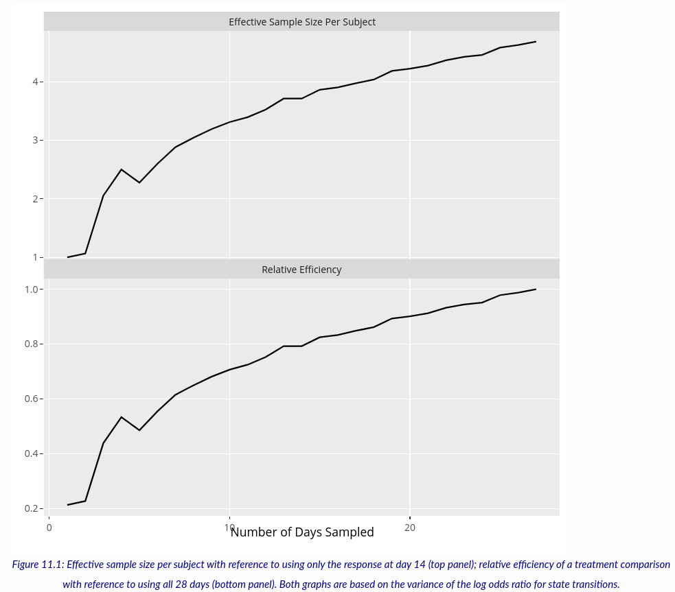
From the top panel, the effect of using all the daily measurements compared to using the ordinal scale on just day 14 is a 4.7 fold increase in effective sample size. In other words, having 27 measurements on each patient is equivalent to having almost 5 \times the sample size if one compares to measuring the outcome on a single day. It would be interesting to repeat this calculation to compare efficiency with time to recovery and support-free days.
In choosing an outcome for a clinical trial, there are several considerations, such as
- relevance to patients
- interpretation by clinicians
- statistical efficiency
- ability of the outcome measure to deal with missing or incomplete data
- elegance with which the outcome measure handles competing/intervening events
- the ability of the main analysis to be rephrased to provide evidence for efficacy on scales that were not envisioned in the primary analysis
Here I make the claim that analysis of the rawest available form of the data satisfies the maximum number of considerations, and importantly, lowers the sample size needed to achieve a specific Bayesian or frequentist power. This is exceptionally important in a pandemic. Lower sample size translates to faster studies. Even though clinical investigators generally believe that time to event or support-free days are more interpretable, this is only because subtleties such as competing events and missing or censored data are hidden from view, and because they are unaware of problems with sample medians when there are ties in the data.
Another exceptionally important point is that one-number summaries hide from view any time-related treatment effects, and they do not shed any clinical light on the time course of these treatment effects. Analysis of serial patient states can use a model that has time \times treatment interaction that would allow for non-constant treatment effect, e.g., delayed treatment effect or early effect that wanes with follow-up time.
One more advantage of modeling the raw data is that missing or partially observed outcome components can be handled in a way that fully respects exactly what was incomplete in the patient’s outcome assessment. For example, if a patient was known to be alive in the hospital on day 6 but organ support was not assessed on day 6, Y is interval censored in [1,2] and the ordinal model’s log likelihood component for that patient-day will use exactly that. On the other hand, how to handle intermediate missing data in time to recovery or support-free days is not clear.
It is important to describe how results of a raw-data-based analysis can be presented. Let’s consider the case where the daily observations are Y=0,1,2,3 as mentioned above. Note that organ support (Y=2) could be further divided into different levels of support that would result in breaking ties in Y=2. I don’t consider that here. Here are some possibilities for reporting results.
- If the serial measurements are modeled with a proportional odds ordinal logistic model, whether using random effects or Markov models to handle within-patient correlation, some consumers of the research will find an odds ratio interpretable. The OR in this context is interpreted the same as the OR in an RCT with a simple binary outcome, it’s just that the outcome being described is outcome level y or worse. If proportional odds holds and the outcome is Y=0,1,2,3, the treatment B : treatment A OR is the odds that a treatment B patient is on organ support or dies divided by the odds that a treatment A patient is on organ support or dies, and is also the odds of dying under B divided by the odds of dying under A. Note odds = P(Y \geq y | treatment) / P(Y < y | treatment)].
- Even if proportional odds is severely violated, the Wilcoxon test statistic, when scaled to be the 0-1 probability of concordance, is \frac{\mathrm{OR}^{0.66}}{1 + \mathrm{OR}^{0.66}}. So the OR is easily translated into the probability that a randomly chosen patient getting treatment B will have a worse outcome than a randomly chosen patient getting A, the so-called probability index or P(B > A).
- Clinicians who like count summaries such as number of support free days will like the expected time in a given state or range of states that comes from a serial state transition ordinal model. For example, one can compute (and get uncertainty intervals for) the expected number of days alive and on a ventilator by treatment (the mean works well because -1 is not being averaged in), the expected number of days alive in hospital and not on organ support, and any other desired count.
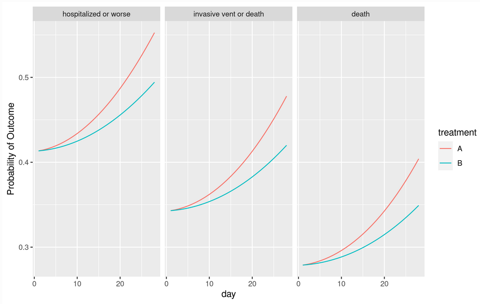
- Natural to many clinicians will be the probability of being in outcome state y or worse as a function of time and treatment (see graph below). This is a function of OR, the proportional odds model intercepts, time, and the serial dependence parameters.
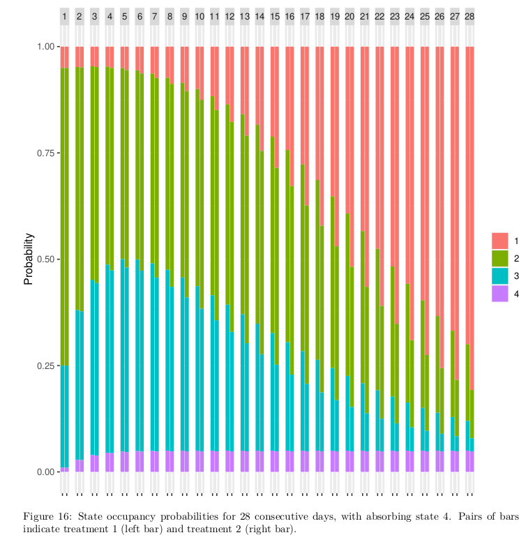
- Equally natural are daily split bar charts showing how treatment B possibly redistributes the proportion of patients in the different outcome states, over time (see below).
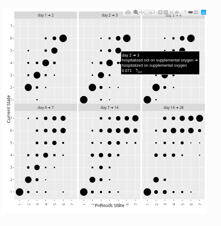
- When using a day-to-day state transition model such as a first-order ordinal Markov model, some clinicians will be interested in state transition probabilities. For example one can easily estimate the probability that a patient on a given treatment who is on ventilator one day will be alive and off ventilator the next day. One can also gain insight by estimating the probability that a patient will return to hospital after being at home 1, 2, 3, …, days, or the probability that a patient will again need a ventilator after going off ventilator.
Here is an example of presenting three outcome probabilities as a function of time and treatment. The model contained a linear time \times treatment interaction, with the treatment having no immediate effect.
Here is a state occupancy probability graph that is becoming more popular in journal articles. TIme is shown at the top, and probabilities for each of two treatments are shown in each pair of bars. This was constructed when the outcomes were coded Y=1,2,3,4.
Here is a snapshot of an interactive state transition chart from the ORCHID study. Go to the link to see how hovering your pointer displays transition details. Transition charts are not “intention to treat” since they represent post-randomization conditional probabilities (much as hazard ratios in Cox models with time-dependent covariates) so they are not featured for final efficacy assessment. But transition charts are closest to the raw data by completely respecting the study design, i.e., by connecting outcomes within individual patients. Thus state transition tendencies are the most mechanistically insightful ways to present discrete longitudinal data.
I argue that
- ordinal longitudinal models are versatile, providing many types of displays of efficacy results as shown in the graphs above
- by using the raw data (other than a slight loss of information when two events occur on the same day, as only the more severe event is used), ordinal longitudinal models such as proportional odds state transition models increase power and thus lower sample size when compared to two-group comparisons of over-time summary indexes
- the types of result displays shown here are actually more clinically interpretable than replacing raw data with one-number summaries, because there are no hidden conditions lurking about, such as missing data or intervening events that interrupt the assessment of the main event of interest
I hope that we can have a robust discussion here, and I would especially appreciate clinical investigators posting comments and questions here. Particular questions about longitudinal ordinal analysis will help us better describe the method.
Resources
- COVID-19
- Articles on ordinal serial outcome analysis
- Articles on Markov models
- Articles on longitudinal analysis in general
