Should one derive risk difference from the odds ratio?

AndersHuitfeldt · January 31, 2022, 11:38am

You are right that I used the wrong number when I calculated the probability of treatment among those with severe disease. I have edited the post. However, this does not affect the argument.

If I understand correctly, you are now saying that disease severity is downstream from randomization, i.e. that it is a mediator rather than a baseline covariate. With this interpretation, you are going to have to deal with very tricky problems that arise from selection bias, as you are conditioning on a post-baseline covariate. I don’t think it will be possible to give this a complete treatment without extensive use of counterfactuals or DAG models. The basic problem is the same as what I described for the case of baseline covariates: You have essentially just found the point where the non-collapsibility of the causal odds ratio is cancelled out by selection bias due to conditioning on a mediator.

HuwLlewelyn · January 31, 2022, 12:32pm

Thank for correcting your probability. It drew my attention to my typo of 0.374 that I have corrected to 0.384!

What I am saying is that disease severity is often affected by treatment, in which case we have to use the odds ratio model theoretically. If it is not affected then the risk ratio model can be applied theoretically. I have to emphasise that the exchangeable groups post randomisation and their baseline covariate proportions cannot be assumed to be the same after any intervention. This is particularly so when two or more active treatments are being compared. It might even be possible that a placebo might change baseline values. It is an over-simplification to assume otherwise. In other words, by applying different interventions or controls we have to assume that we are creating new counterfactual sets.

AndersHuitfeldt · January 31, 2022, 12:46pm

Baseline covariates are defined in terms of the value that the underlying construct had at baseline. The covariates do not change post-baseline, no matter what the intervention is. We condition on the baseline value of the covariate, and define strata based on the value that the covariate had at baseline. With proper randomization, baseline covariates will (in expectation) be balanced across randomization arms.

AndersHuitfeldt · February 2, 2022, 2:05pm

Our talk at the Berlin Epidemiology Methods Colloquium is happening in 55 minutes. Sign up at Webinar Registration - Zoom

mshapiro123 · February 3, 2022, 8:53pm

Catching up on this never-ending thread after a couple of months and it never disappoints!

HuwLlewelyn · July 8, 2022, 2:26pm

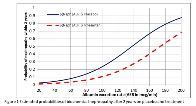
I have been reflecting further on this issue of whether we should estimate the risk differences from the risk ratio or odds ratio obtained from RCTs. I want to explain these issues to medical students, trainee doctors (and hopefully readers from other disciplines) in the final chapter of the forthcoming 4th edition of the Oxford Handbook of Clinical Diagnosis. I have had to conclude that neither the risk ratio nor odds ratio obtained from a RCT can be used to estimate the absolute risk reduction for different baseline risks. I used the data from the IRMA 2 study to fit logistic regression curves to the estimate risks of nephropathy in patients with different albumin excretion rates on placebo and treatment. The result is shown in Figure1.

I then found the risk difference, the risk ratio and odds ratio at each point on these curves. As shown in Figure 2, neither the risk ratio nor the odds ratio was constant for all baseline risks provided by the placebo curve providing a counter-example for the constancy of both.

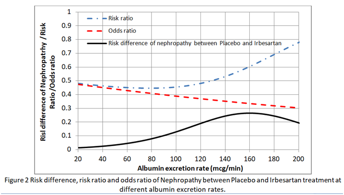
This implies that in order to estimate the absolute risk reduction, baseline data that predict risks of nephropathy have to be recorded during the RCT (e.g. as in the IRMA 2 study). Ideally the effects of covariates such as BP and HbA1c (that reflects blood glucose control) have to be minimised in the RCT so that the baseline risks are as low as possible (e.g. 0.01 to 0.02 at 20mcg/min in Figure 1). If the baseline risk in an individual patient is high (e.g. 0.5 at an AER of 100mcg/min due to for example additionally uncontrolled hypertension or uncontrolled diabetes), then the appropriate risk reduction (e.g. of 0.13 at an AER of 100mcg/min in Figure 2) is subtracted from this high individual baseline risk to give the new risk on treatment (e.g. of 0.5-0.13 = 0.37). Note that the risk ratio of 0.11/0.24 = 0.46 at an AER of 100mcg/min should not be applied to the total risk as this would exaggerate the effect of treatment by suggesting that the new risk was lower at 0.5x0.46= 0.23 as opposed to 0.37. This is common practice - applying risk ratios to total risk (e.g. when a risk ratio from RCTs on statins is applied to cardiovascular risks based on age, high BP, diabetes etc).

I would be grateful for comments.

s_doi · July 8, 2022, 10:17pm

Interesting question you have posed Huw. In your example, intervention is ARB, outcome is nephropathy development at two years and the third variable is AER. If you were to plot the outcome probability under no-ARB on the X-axis and outcome probability under ARB on the Y-axis for different levels of AER, and if these probabilities were derived from a GLM with log, logit and identity links, what you would find is that the plot would be linear for log and identity links and ROC like for the logit link derived probabilities. You can decide for yourself which is valid once you create these plots and it would be great if you could post them here once created as those will be more informative for this discussion. .

Regarding portability over baseline risk for an effect measure - you have taken that literally to mean that the predicted probabilities from a model should return the same magnitude of effect at every level of the third variable (constancy). What we mean when we talked about portability in our paper is that the value of baseline risk has no mathematical implication for the magnitude of effect and not what you have assumed it to mean. If you look back at our paper that started this thread you will note that the OR shows no trend across multiple trials with different baseline risks so obviously there is no direct mathematical influence of baseline risk on it. This is not the case for the RR or RD.

f2harrell · July 8, 2022, 11:09pm

If the odds ratio is not constant that means there is an interaction between treatment and AER in the logistic model. The interaction needs to be taken into account when computing ARR or RR.

The basis to emphasize (ARR, RR, OR) needs to come from an assimilation of hundreds of trials in the literature. Which measure is the most constant over subgroups? My money is on the OR.

HuwLlewelyn · July 9, 2022, 12:49pm

Thank you @S_Doi. Here is the plot of p(Neph|AER&Placebo) against p(Neph|AER&Irbesartan). It is not linear of course.

However, the expressions for Excel’s 6 order polynomials fitted to these curves are displayed on Figure 4 below (the top one is for placebo) so that you can re-construct these curves to explore different plots if you wish.

The plot of AER against ln(odds)(Neph|AER&Placebo) and AER against ln(odds)(Neph|AER&Treatment) as the first step in calculating the logistic regression are both linear of course. It follows that the plot of ln(odds)(Neph|AER&Placebo) against ln(odds)(Neph|AER&Treatment) is also linear. Little else seems to be linear including the plot of AER against odds (it is a gentle curve) and AER against risk ratio as shown in Figure 2 of my previous post.

s_doi · July 9, 2022, 4:05pm

Yes, that is what we expect with predicted probabilities from logistic regression - the curve in Fig 3 is below the central diagonal line because ARB is protective and the area under the curve is a measure of the interventions ability to discriminate between those that will or will not develop the outcome.

I have computed a similar plot from the GUSTO-I trial where X is hypotension at presentation, Y is day 30 mortality and Z is Killip class (four levels). Below is what we find from the three models:

three plots

As can be seen, only a logit link allows the bending of the predicted probabilities so that at the extremes of the ranges they come together (as expected) without impacting the magnitude of the effect measure. The other two effect measures will only meet this required behavior if the effect magnitude is modified across baseline risk otherwise they will end up predicting impossible probabilities.

HuwLlewelyn · July 9, 2022, 4:32pm

If the odds ratio is not constant that means there is an interaction between treatment and AER in the logistic model. The interaction needs to be taken into account when computing ARR or RR.

Thank you @f2harrell. If we have an RCT result where the proportion with an outcome on placebo is 0.4 and on treatment it is 0.2, the RR is 0.5 and the OR is 0.375. If an individual’s disease severity is S and the baseline risk at this disease severity is 0.8, then assuming a constant RR, the reduced risk on treatment is 0.8x0.5=0.4. However if the OR is constant then the reduced risk on treatment is 0.6.

If the likelihood of disease severity ‘S’ conditional on the outcome O is p(S|O)= 0.6, then the probability of someone in the trial having the severity S on placebo is

p(S) = p(O).p(S|O)/p(O|S) = 0.4x0.6/0.8 = 0.3.

If we assume a constant RR then the probability of someone in the trial having the severity S on treatment is also

p(S) = p(O).p(S|O)/p(O|S) = 0.2x0.6/0.4 = 0.3.

This is what we expect as randomisation should allow patients with similar degrees of severity to be present in both limbs of the RCT.

However, if we assume a constant OR then p(O|S) is now 0.6 so the probability of someone having the severity S on treatment is

p(S) = p(O).p(S|O)/p(O|S) = 0.2x0.6/0.6 = 0.2.

This means that the proportion of individuals with disease severity ‘S’ in the treatment limb is different from that in the control limb. This shows that when we use the OR model then we model interaction with disease severity (represented by the albumin excretion rate or AER in my example).

This is why I decided to fit a logistic regression functions independently to the treatment and placebo data. I was therefore able to illustrate the point that neither the RR nor OR are suitable for estimating the outcome probability of treatment from the baseline probability (e.g. on placebo).

The basis to emphasize (ARR, RR, OR) needs to come from an assimilation of hundreds of trials in the literature. Which measure is the most constant over subgroups? My money is on the OR

I agree that the OR is a better summary of efficacy than the RR. The OR and RR are of course similar at low probabilities but the RR gives bizarre results at higher probabilities. The OR should therefore give more consistent summary results across subgroups, as you say, especially if the average baseline risks vary between individual trials. However the OR as estimated in a RCT appears to be a summary of the range of different ORs at different baseline risks largely due to different severities of disease. I am very interested as a clinician in these degrees of severity and estimating accurately their effect on treatment efficacy in the form of absolute risk reduction, which is why I think it is more appropriate to fit logistic regression functions independently to the treatment and placebo data.

s_doi · July 9, 2022, 5:46pm

If the likelihood of disease severity ‘S’ conditional on the outcome O is p(S|O)= 0.6, then the probability of someone in the trial having the severity S on placebo is

p(S) = p(O).p(S|O)/p(O|S) = 0.4x0.6/0.8 = 0.3.

It is not clear what you have calculated here - please explain

HuwLlewelyn · July 9, 2022, 6:40pm

I tried to set up a simplified example where the p(O) in the placebo limb of an RCT was 0.4 and p(O) in the treatment limb was 0.2. This provides a RR of 0.2/0.4 = 0.5 and an OR of (0.2/0.8)/(0.4/0.6) = 0.375. I then proposed that a subset of those in the trial with the finding S provided a conditional probability of p(O|S) = 0.8 and p(S|O) = 0.6.

From Bayes rule: p(O|S) = p(O).p(S|O)/p(S)

Rearranging: p(S) = p(O).p(S|O)/p(O|S)

So that p(S) = 0.4x0.6/0.8 = 0.3

s_doi · July 9, 2022, 7:26pm

I don’t think we can use Bayes’ rule with the third variable and the outcome if we want to interpret the trial in diagnostic terms. For that we need to assume the outcome is a “test” of the intervention status. Thus we have the following from Bayes’ rule:
P(ARB|O)/[1-P(ARB|O)] = [P(O|ARB)/P(O|no-ARB)] × [P(ARB)/(1-P(ARB))]
Where [P(O|ARB)/P(O|no-ARB)] = RR
See the full exposition here: The likelihood ratio interpretation of the relative risk

HuwLlewelyn · July 10, 2022, 9:30am

Thank you @S_Doi. I too would be grateful for clarification. By ’No ARB’ do you mean Control (e.g. Placebo)? If this is the case and there is randomisation to treatment or control then the probability of ending up on treatment should be approximately the same as the probability of ending up on control (i.e. approximately 0.5) so that:

P(ARB) ≈ (1-P(ARB))

so that P(ARB|O)/[1-P(ARB|O)] ≈ [P(O|ARB)/P(O|no-ARB)].

Do you agree?

My application of Bayes rule was different and was applied to two counterfactual sets: (1) the set of patients randomised to treatment and (2) the set of patients randomised to control. Also my intention was not to use the outcome as a diagnostic test to estimate the odds that the patients had been randomised to treatment as in your case. My intention was to estimate the probability of an outcome on treatment, the probability of the outcome on control and also how disease severity affects these estimated probabilities. These probabilities are used with other information (e.g. about adverse effects) to make a decision about whether to offer the treatment or not.

s_doi · July 10, 2022, 1:19pm

Yes, I agree - if there is 1:1 randomization then the prior odds is 1 so that the posterior odds equals the likelihood ratio

Let us take your example:
Control risk =0.4
Treatment risk = 0.2
LR(nephropathy) =0.5 and LR(no-nephropathy)= 0.8/0.6=1.33 .
If we use Bayes’ theorem we can connect the new no-ARB risk (0.8) to the expected ARB risk using the ratio of the LR’s = 0.5/1.33 =0.375
The individual’s disease severity alters baseline risk only (if it is not an effect modifier) and new baseline risk = 0.8 (and odds = 4)
So ARB odds = 4 * 0.375 = 1.5 and ARB risk is 1.5/2.5 = 0.6
Note that the new RR at this severity is 0.6/0.8 = 0.75 (not 0.5)
Had we used the non-Bayes’ method then:
ARB risk = 0.8*0.5 = 0.4 which is obviously wrong

HuwLlewelyn · July 10, 2022, 10:05pm

Thank you again @S_Doi for your comments. I think that you may have misinterpreted my example. When C is control, T is treatment, O is a particular outcome, S is a particular degree of severity then my understanding is as follows:

If p(O|C) = 0.4, p(O|T) = 0.2, p(T) = 0.5, p(C) = 0.5, RR= 0.2/0.4 = 0.5 and OR = 0.375,
Then p(C|O) = 1/(1+ p(T)/p(C) * p(O|T)/p(O|C))= 1/(1+ (0.5/0.5) (0.2/0.4)) = 0.67
and p(T|O) = 1/(1+ p(C)/p(T) * p(O|C)/p(O|T))= 1/(1+ (0.5/0.5) (0.4/0.2)) = 0.33

If p(O|C&S) = 0.8 and we apply the model of constant odds ratio to estimating the effect of the degree of severity ‘S’ then OR = (0.2/0.8)/(0.4/0.6) = 0.375 so that NOW p(O|C&T) = (0.8/0.2 x 0.375)/(1+ (0.8/0.2 x 0.375)) = 0.6 ,
Then p(C|O&S) = 1/(1+ p(T)/p(C) * p(O&S|T)/p(O&S|C))= 1/(1+ (0.5/0.5) (0.6/0.8)) = 0.57
and p(T|O) = 1/(1+ p(C)/p(T) * p(O&S|C)/p(O&S|T))= 1/(1+ (0.5/0.5) (0.8/0.6)) = 0.43

In other words if we apply different models to estimate the effect of disease severity on treatment effects, we get different results. This affects the above calculated probability of whether a patient had been treated or given a control conditional on the outcome. The point of my post is that neither the RR nor the OR models are satisfactory for this purpose and that perhaps we should fit logistic regression functions to treatment and control data.

However as @r2harrell points out, if we wish to compare treatment efficacy between RCTs (e.g. during a meta-analysis) then the OR gives a more consistent result than RR.

s_doi · July 10, 2022, 11:35pm

Thanks @HuwLlewelyn. Before we proceed to the next step lets examine the first:
if O is a particular outcome and nO is its complement then:
LR(O) = p(O|T) / p(O|C) = 0.5 and LR(nO) = [1- p(O|T)]/[1- p(O|C)] = 1.33
so I agree that p(T|O) = 0.5/1.5 = 0.33 and p(C|O) = 1 - 0.33 = 0.67
but p(T|nO) = 1.33/2.33 = 0.57
This has to be correct because 1.33 × 0.375 = 0.5 where 0.375 is the OR - Do you agree?
I don’t get the next part - the only role S should have is to change p(O|C) to 0.8 from 0.4 hence the use of p(O|C,S) = 0.8. Then (from conventional wisdom that I do not agree with) it follows that p(O|T,S) = RR×0.8 = 0.4
So far it seems clear but please explain what followed:
“Then p(C|O&S) = 1/(1+ p(T)/p(C) * p(O&S|T)/p(O&S|C))= 1/(1+ (0.5/0.5) (0.4/0.8)) = 0.67
and p(T|O) = 1/(1+ p(C)/p(T) * p(O&S|C)/p(O&S|T))= 1/(1+ (0.5/0.5) (0.8/0.4)) = 0.33”

Addendum 2
Edited based on the next post

HuwLlewelyn · July 11, 2022, 6:57am

But p(C|O) + p(T|O) = 1
So p(C|O) =1- p(T|O) = 1 - 0.33 = 0.67 (not 0.75)

s_doi · July 11, 2022, 7:50am

You are right - they must add to 1. When I look back I realize that what I put as p(C|O) in the previous post is actually p(T|nO). I will edit this and put the changes in bold and then respond again after I think this through