Individual response

I am not sure what Judea Pearl was trying to do by offering this example based on alleles and tasty medication. His and Scott’s paper contains the necessary data to illustrate their argument of how to place bounds on the probabilities of 4 counterfactual situations of (1) survival on control and treatment (2) no survival on control but survival on treatment (‘benefit’), (3) survival on control but not on treatment (‘harm’) and non-survival on control and treatment. I proposed one hypothetical narrative that would make sense of their data from a clinical point of view (see Individual response - #65 by HuwLlewelyn). With imagination, there could be many such appealing narratives but the allele / tasty drug example as proposed by Judea Pearl does not appear to be one of them.

It seems to me that dreaming up appealing illustrative narratives is not the issue. From my viewpoint there are 4 important questions:

  1. The paper’s use of the word ‘benefit’ and ‘harm’ in a counterfactual situation differs from that used when describing the probabilities of an outcome conditional on control and treatment and designating the treatment beneficial or harmful.
  2. If we could derive probabilities for the above, how would they be used to make medical decisions by also taking into account probabilities of adverse effects and their various utilities (i.e. effects on well-being)? In other words, what is the purpose of calculating probabilities of these 4 counterfactual situations?
  3. They are estimating the probabilities of counterfactual situations that are by definition inaccessible for the purposes of verification or calibration, unlike other models of prediction for example.
  4. In view of (3) are their assumptions and reasoning about using various results from RCTs and observational studies to arrive at inequality probabilities of these counterfactual situations sound, culminating on page 8 of the paper?
3 Likes

@Pavlos_Msaouel I want to rethink this and disagree with you a bit.

The problem with overall survival (OS) in oncology studies stems solely from the existence of rescue therapy that can prevent or delay death (and can also prevent cancer recurrence but we are talking mainly about post-recurrence changes in therapy). I posit that most any method that tries to estimate OS will be hard to interpret. The only easy clinical interpretation comes from estimating things like the probability of either the need for rescue therapy or death. A state transition model can easily distinguish between need for rescue therapy with and without a later death, and it can count death as worse than rescue therapy. State occupany probabilities can be computed, by treatment, for death, rescue tx or death, rescue tx and alive, etc.

1 Like

Love it! Obviously there are currently differences but this is an open problem and glad to see you using your skills and experience to address it your way.

In fact, if I recall correctly, part of the motivation for writing that DFS vs OS post at the time was that you had posted a comment on another datamethods thread at the time talking about your state transition model approach in the context of COVID-19 trials. Intuitively I can see connections but unable to go deeper, in part also because the cancer that truly motivates my research (renal medullary carcinoma) is highly aggressive and we are not yet at the point therapeutically where we need to use new methods for survival estimation. Thus, I think about this topic far less than I do other challenges.

While our team has very elaborate and efficient Bayesian non-parametric models we use to attack this problem, it is not certain that they will be the optimal approach. A major reason why is that they are time-consuming, hard to intuit/interpret, and lack user-friendly tools. On the other hand, you are an expert with decades of experience at creating popular and powerful modeling tools for the community. Would love to see your group approach these problems.

1 Like

Thanks Pavlos. Ordinal longitudinal Markov state transition models have lots of advantages of interpretation as detailed here, besides being very true to the data generation process. Advantages come from the variety of causal estimands through the use of state occupancy probabilities, and the fact that all of these estimands are simple unconditional (except for conditioning on treatment and baseline covariates) probabilities. What I thin k is needed to make this work in your context are

  • rescue therapies must have a clinical consensus around them to be considered for the list (and note that you can distinguish various levels of “rescue” with an ordinal outcome, e.g. surgical vs chemo vs radiation vs chemo+rad)
  • in a multi-center RCT the practice patterns for use of rescue therapy are fairly uniform or can be somewhat dictated by a protocol

To me the only problems that are really hard to solve in this context are the existence of non-related follow-up therapies and non-related causes of death such as accidental death.

1 Like

I think these excellent considerations deserve an ongoing discussion/panel particularly with regulators such as the FDA because the challenge is becoming progressively more common across diseases.

Right now I’m trying to start just such a project at FDA but for neurodegenerative disease.

Presently at FDA rescue therapy is somethat that is worked around rather than directly addressed, thinking of it as more of a censoring event than an outcome. That always makes results hard to interpret to me.

1 Like

I have gone over the paper again carefully. The assumption on which the whole paper is based is ‘consistency’. To quote from the paper: “At the individual level, the connection between behaviors in the two studies relies on an assumption known as ‘consistency’ (Pearl, 2009, 2010), asserting that an individual response to treatment depends entirely on biological factors, unaffected by the settings in which treatment is taken. In other words, the outcome of a person choosing the drug would be the same had this person been assigned to the treatment group in an RCT study. Similarly, if we observe someone avoiding the drug, their outcome is the same as if they were in the control group of our RCT. In terms of our notation, consistency implies: P(yt|t) = P(y|t), P(yc|c) = P(y|c).”

However, according to their example data for females:
P(yt|t) = 489/1000 = 0.489, P(y|t)= 378/1000 =0.378, P(yc|c) = 210/1000=0.210, P(y|c)=420/600 = 0.7
So that P(yt|t) ≠ P(y|t), P(yc|c) ≠ P(y|c)

According to their example data for males:
P(yt|t) = 49/1000 = 0.49, P(y|t)= 980/1400 = 0.7, P(yc|c) = 210/100=0.210, P(y|c)=420/600=0.7
So that P(yt|t) ≠ P(y|t), P(yc|c) ≠ P(y|c)

This means that the assumption of consistency is not applicable to the paper’s example data of their RCT and observational study. However, they go on to make the calculations nevertheless “based on this assumption (i.e. of ‘consistency’), and leveraging both experimental and observational data, Tian and Pearl (Tian and Pearl, 2000) derived the following tight bounds on the probability of benefit, as defined in equation (3): P(benefit) = P(yt, y′c). Therefore the estimated probability bounds in their inequality equation (5) do not follow from their assumptions and reasoning. However, by applying these probability bounds they arrive at point estimates of the probability of counterfactual ‘benefit’ and ‘harm’ (the latter are defined in my previous post (Individual response - #205 by HuwLlewelyn).

I created new example data for males and females where the RCT data were identical and the proportions choosing to take the drug and not to take it were the same as in their observational example. However in my new observational study data, P(yt|t) = P(y|t) and P(yc|c) = P(y|c) so that the assumption of ‘consistency’ could be applied. I then applied their calculations to this data that I had created.

Instead of getting point estimates I got probability ranges. For females the probability of ‘benefit’ counterfactually (e.g. by giving treatment, turning the clock back and giving placebo) was between 0.279 and 0.489 and the probability of ‘harm’ was between 0 and 0.21. For males the probability of ‘benefit’ was between 0.28 and 0.49 and the probability of ‘harm’ was between 0 and 0.21. (p(Harm) = p(Benefit) – CATE, which was 0.279 and 0.28 for females and males respectively). The calculations are in the Appendix below. If the assumption of consistency is valid, we can tell all this from the RCT alone: p(Benefit) ≥ Pr(yt) - Pr(yc) and P(Benefit) ≤ Pr(yt) and p(Harm) = p(Benefit) - (Pr(yt) - Pr(yc)), so that the observational study adds nothing in this context. As we have discussed already, observational studies can be useful in other ways such as detecting adverse effects.

Appendix
Female RCT and ‘consistent’ observational study

Calculations for females (replacing those on pages 8 and 9 in the paper), when Pr indicates that the probability is from the RCT and Po indicates that the probability is derived form the observation study:
P(Benefit) ≥ 0
P(Benefit) ≥ Pr(yt) - Pr(yc) = 489/1000 -210/1000 = 279/1000 = CATE = 0.279
P(Benefit) ≥ Po(y) - Pr(yc) = 0.4053 – 0.21 = 0.1953
P(Benefit) ≥ Pr(yt) - Po(y) = 0.489-0.4053 = 0.0807

P(Benefit) ≤ Pr(yt) = 489/1000 = 0.489
P(Benefit) ≤ Pr(y’c) = 790/1000 = 0.79
P(Benefit) ≤ Po(t, y) + Po(c, y’) = 686/2000 + 474/2000 = 0.343 +0.237 = 0.58
P(Benefit) ≤ Pr(yt) − Pr(yc) + Po(t, y′) + Po(c, y) = 0.489-0.21 +0.357+0.063 = 0.6997
Therefore:
0.279 ≤ p(Benefit) ≤ 0.489 and (0.279-0.279) = 0 ≤ p(Harm) ≤ 0.21 = (0.489-0.279)

Male RCT and ‘consistent’ observational study

Calculations for Males (replacing those on pages 8 and 9 in the paper):
P(Benefit) ≥ 0
P(Benefit) ≥ Pr(yt) - Pr(yc) = 490/1000 -210/1000 = 280/1000 = 0.28 = CATE = 0.28
P(Benefit) ≥ Po(y) - Pr(yc) = 0.406 – 0.21 = 0.196
P(Benefit) ≥ Pr(yt) - Po(y) = 0.49-0.406 = 0.084

P(Benefit) ≤ Pr(yt) = 49/1000 = 0.49
P(Benefit) ≤ Pr(y’c) = 790/1000 = 0.79
P(Benefit) ≤ Po(t, y) + Po(c, y’) = 686/2000 + 474/2000 = 0.343+0.237 = 0.58
P(Benefit) ≤ Pr(yt) − Pr(yc) + Po(t, y′) + Po(c, y) = 0.49-0.21 +0.357+0.63 = 0.7

Therefore:
0.28 ≤ p(Benefit) ≤ 0.49 and (0.28-0.28) = 0 ≤ p(Harm) ≤ 0.21 = (0.49-0.28)

4 Likes

I agree. To use the words of Gelman, I think it’s helpful to develop statistical methods in the context of applications, and also to work toward theoretical understanding, as Pearl has been doing. However, the push towards theoretical understanding from Pearl has been around for a long time yet it lacks any concrete practical application (except for the theoretical ones like in this thread). No clinician in this thread so far has endorsed any of this as helpful for clinical decision making so I wonder where we are heading? It would be good if someone on this thread could post a real world example of where a problem has been solved using the theoretical explanations posted in this thread.

2 Likes

Thank you @s_doi. There seem to be many reasons for the failure to implement these theoretical ideas. One is difficulties in communication. For example, ‘benefit’ and ‘harm’ as an individual response in the context of counterfactual situations has a completely different meaning to benefit and harm arising from the use of an intervention. This is illustrated in the paper’s conclusion that in females the probability of individual ‘harm’ from treatment is zero when more people die on the treatment than on placebo. The latter describes the response of groups of individuals and is subject to stochastic variation, which as @Stephen pointed out, prevents estimation of individual response. The probabilities of outcomes can be substantiated by experiment whereas we cannot in reality turn the clock back and create a counterfactual situation to substantiate individual response.

We have a rationale for making decisions based on outcome probabilities but it not clear how probabilities of ‘individual benefit’ or ‘individual harm’ would change these decisions. From my calculations, it does not change the information available to us from RCTs at all as p(Benefit) ≥ Pr(yt) - Pr(yc) and P(Benefit) ≤ Pr(yt) and p(Harm) = p(Benefit) - (Pr(yt) - Pr(yc)). What we need is better predictive information (e.g. when everyone dies by using parachute with a big hole in the canopy but no one dies with a proper parachute). In this situation an observational study would be as good as an RCT but reason alone as good as both, making the studies unethical! However, the reasoning must be sound, which includes checking that the assumptions about the data are consistent with the data (or at least not clearly inconsistent).

3 Likes

Thanks @HuwLlewelyn , I think your summary brings great clarity to this discussion and makes a lot of sense. It also reminds me of a quote in some other thread attributed to Vineet Tiruvadi that seems to apply to the framework in this thread “if you start with the wrong framework then the ability to do complex analyses may seem like it’s giving insight, but what you’re mostly doing is studying how wrong your framework is

2 Likes

This discussion is incredibly helpful. @HuwLlewelyn joins @Stephen Senn in being the most impressive scientists I’ve known in their abilities to cut through arguments of others and to make cogent new arguments. It confirms what @Stephen has argued repeatedly that principles of experimental and clinical trial design must be brought to causal inference about treatment effects. The discussion also confirms my previous feeling that outside of special situations (such as analysis of treatment effects within RCTs compensating for non-adherence to treatment) causal inference remains a theoretical nicety and a great thought organizer but has not yet been translated to practical application in treatment evaluation. Hence the lack of uptake on the challenge put at https://discourse.datamethods.org/t/examples-of-solid-causal-inferences-from-purely-observational-data.

6 Likes

One area where causal inference might be translated to a practical application in treatment evaluation is when taking HTE into consideration. This was a tweet that I addressed to Judea Pearl recently to which he did not reply:

In RCTs Irbesartan reduces risk of nephropathy. HbA1c & AER are risk factors. According to ‘causal’ medical theory, Irbesartan should reduce AER but not HbA1c. For HTE, should risk reduction be estimated due to that of AER alone & not HbA1c? How does CI notation express this?

How would @Stephen and others in this discussion design a study to answer this question?

I have yet to study Huw’s reply in detail but on a brief read I think that it gets to the nub of the argument. It seems baffling to me that consistency is considered to be reasonable or practical. However, I wonder if in fact M&P depends on more than just “that an individual response to treatment depends entirely on biological factors, unaffected by the settings in which treatment is taken”. The individuals contributing information from the observational studies are not the same individuals as in the RCTs. Thus we have to be able to assume that the two sets of individual are exchangeable to the extent needed in order to be able to solve for the unknowns. I do not consider this to be a reasonable assumption and referred to “study effects” as being a problem. The TARGET study is an excellent example of the problem Lessons from TGN1412 and TARGET: implications for observational studies and meta‐analysis - Senn - 2008 - Pharmaceutical Statistics - Wiley Online Library
The way that study effects are dealt with in conventional statistical approaches is either by declaring them as fixed and hence eliminating them by contrasts or as declaring them as random and then trying to estimate the variance component. All of this was extensively developed in connection with incomplete block designs by the Rothamsted school in the period 1925-1945.
My view is that adding observational data does not pull the rabbit out of the hat. Adding extra equations does not necessarily render a system identifiable, in particular, if in doing so one adds more unknowns.

5 Likes

I would like to sum up following @Stephen’s and my latest skirmish with Judea Pearl on Twitter. He wrote that I was wrong to assume that p(Yt) from the RCT should have been equal to p(y|t) from the observation study. However he reasserted that p(y|t) was equal to p(yt|t), the latter being the result of a ‘Level 3’ or imaginary RCT result that applies to choosers (it can be imagined after reasoning from other established beliefs but cannot be done in realty). It seems that the assumption of ‘consistency’ is therefore a Level 3 or imagined result of p(yt|t) that is equal to (y|t) the observation study result. This assumption of ‘consistency’ is therefore unverifiable and un-refutable by study and based on personal belief leading to a forceful assertion.

The only probabilities supported by reliable data are the results of the RCT. If we are only prepared to rely on the RCT results (but not rely on forceful assertions based on imagination) then all we can conclude is that from counterfactual concepts, p(Individual Benefit) ≥ Pr(yt) - Pr(yc) and P(Individual Benefit) ≤ Pr(yt) and p(Individual Harm) = p(Individual Benefit) - (Pr(yt) - Pr(yc)) as I explained in a previous post. However, the latter probabilities of imaginary individual counterfactual outcomes do not seem to make any difference to practical decisions, which result in the reasoning set out in @Stephen’s Twitter response [See https://twitter.com/stephensenn/status/1617807975858704385?s=20&t=8Kkuwt3CM9K7ceCUYGnSXA].

1 Like

Huw, I and others greatly appreciate your diligence on this incredibly important topic. I tried my very best to get Judea to join us here so that he could try to expand his arguments and provide details as you have done, and also to carefully read all the posts here, but to no avail. But your posts, like those of @Stephen are also highly useful for citing in tweets. If you haven’t done this already, clicking on the 3 dots at the bottom of the post pulls up a chain link symbol that can be clicked on to get the URL that leads directly to a specific reply, for inclusion in a tweet.

I agree that it is a pity that Judea Pearl does not engage in our discussions on this site. I suppose he can still follow links to find out what we are writing; I will link my Twitter posts to this site more consistently from now on! He has now responded in a general way this morning to my question about how to verify his assumptions about consistency and I have asked for a link or reference to his source. You will have learnt from my recent post on ‘solid causal inferences’ [Examples of solid causal inferences from purely observational data - #26 by HuwLlewelyn] that I have spent a lot of thought and time on how we can use post licensing ‘observational’ studies learn how to apply RCT results to patient care and to monitor our effectiveness. I am hoping that my diligence in participating in these discussions will help me to learn how best to explain my own ideas to the statistical and CI communities (as in addition to clinicians in my own community).

1 Like

@Pavlos_Msaouel - this new R package is relevant: Multi-State Models for Oncology

Very nice. Would prefer if the survival curves show the confidence bands for the difference as per your approach, e.g., here.

You may also find interesting how we modeled disease status here in an oncology phase I-II design scenario.

“If you are referring to the example in our paper, then my conclusion is somewhat different: The FDA should license the drug for all females and lounch (sic) a study to explore the existence of features E and F that produce benefit in some males and harm in others.”

I’d love to see how this would work in practice. It’s a shame the author won’t engage here to describe his proposal further.

Mathematics is not MY TERMS or YOUR TERMS, it is a useful language to communicate ideas unambiguously, even across disciplines.

Strong disagree. This statement is only true when all important and relevant stakeholders are able to communicate with, and understand, math and symbols- and the pool of such people is very small indeed.

Communicating in math and symbols is a great way to alienate a huge swathe of relevant stakeholders who might otherwise be able to identify major conceptual blindspots. Ultimately, the rate-limiting step in the process of getting any idea implemented is the ability to make ourselves understood by others…

I will argue here that those males and females in the observation study must have been given advice based on the results of the RCT and that all the required information would have been available from the RCTs so that the observation study is not required. However, the RCT results had to be re-constructed by working backwards from the observation study. I will also address the point made by @ESMD that mathematical symbols should be linked to verbal reasoning in order to broaden discussions to make use of broader expertise.

The assumption that allowed this reconstruction was that the proportion of patients dying on no treatment in the observation study was the same as in the RCTs. Similarly, the proportion surviving on treatment in the observational study was in the same as in the RCT. This information can therefore be used to reconstruct what would have happened in the RCT if information about the nature of treatment was not available or had been withheld from the participants so that potential treatment choosers as well as those refusing had been randomised to be given treatment or no treatment.

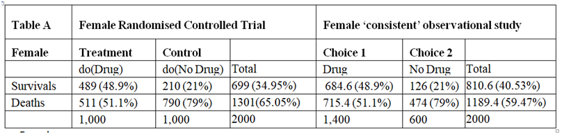
There was clearly a big difference in the outcome of those patients choosing to take the treatment in the observational studies compared to those refusing, suggesting that it was not due to chance from some random or uninformed choice. This suggests that during the observational study, the choice was informed and based on advice as a result of what was discovered in the RCTs (or less likely known before the RCT was done but unethically withheld from the patients agreeing to participate). It can therefore be assumed that this knowledge would not have been available before the RCTs on females and males otherwise those patients who would be harmed or not helped significantly would have been excluded.

Disease severity is always known in patients recruited into a RCT. Those with minimal disease or very severe disease are usually excluded. Typically those with severe disease feel more uncomfortable and develop an unwanted outcome (e.g. death) more often than those with less severe disease and given the choice they would opt for treatment. For the sake of argument, the label {s} for severe will be applied to those who chose treatment in the observation study. However, the patient characteristic represented by {s} might have been something different (e.g. a known gene, DNA pattern or family history of anaphylaxis).

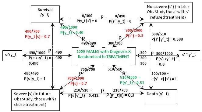
Figure 1 is what I call a ‘P Map’ that I use in my teaching and in the Oxford Handbook of Clinical Diagnosis to try to translate verbal reasoning with probabilities into mathematical symbols. The arrows represent probabilities statements e.g. in Figure 1 the top arrow from right to left states that ‘Of those with ’ Not Severe’ {s’} a proportion / probability of 210/300 = P(y_c|s’) = 0.7 lead to Survival (y_c)'. The remainder of Figure 1 represents the proportions and probabilities arising from those male and female participants who were randomised to the control (no treatment) group in the RCTs. They are represented by one figure because the results were identical for males and females.

Figure 1: The results of randomisation to control group in the RCTs on males and females
Figure 1e

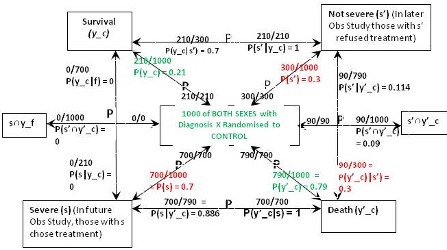
Referring to the notation in Figure 1, we know from the RCT that P(y_c) = 0.21, P(y’_c) = 0.79 (see green type). We are told from the Observational Study (see red type) that the feature (s) that prompted choosing treatment occurred in 70% of males and females so P(s) = 0.7 and P(s’) = 0.3. We are also told that the 30% frequency of death in those on no treatment in the Observational Study was the same as in the RCT, so p(y’_c|s’) = 0.3. This information so far allows us to calculate all the other probabilities and proportions in Figure1. Thus from Bayes rule, p(s’|y’)_c = 0.3x0.3/0.79 = 0.114 so that p(s|y’_c) = 1-0.114 = 0.886. From Bayes rule, p(y’_c|s) = 0.79x0.886/0.7 = 1 so that p(y_c|s) = 1 – 1 = 0.

Figure 2: The results of randomisation to the treatment group in the RCT on females

Figure 2e

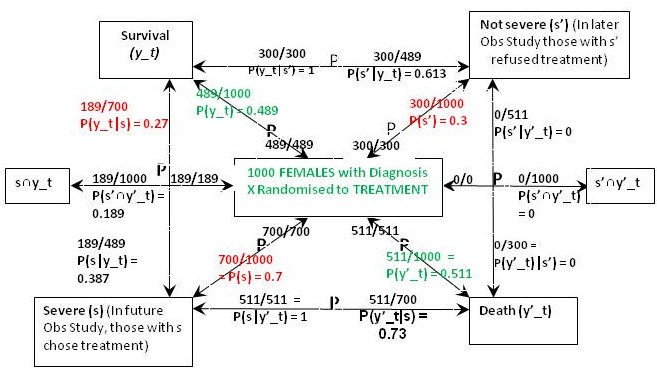
The result of the RCT on females when they were randomised to treatment is shown in Figure 2. This time were told that 27% of those with the feature (s) who chose treatment in the Observational Study would have been the same in the RCT, so in the latter, P(y_t|s) = 0.27 and P(y’_t|s) = 0.73. From Bayes rule, P(s|y’_t) = 0.7x0.73/0.511 = 1 so that P(‘|y’_t) = 1 – 1 = 0 and by Bayes rule, P(s’|y’_t) = 0. This also means that P(s’∩y’_t) = 0 and from Figure 1, P(s’∩y’_c) = 0.09.If p(Benefit) = [P(s’∩y_t)-P(s’∩y_c)]+[P(s∩y_t)-P(s∩y_c)[ = [0.3-0.21]+[0.189-0]=0.09+0.189=0.279, then p(Harm) = p(Benefit)-ATE= 0.279-0.279=0.

The above results means that those with and without feature {s} benefit from treatment by more surviving (and fewer dying) on treatment than on placebo). In other words between subsets {s’∩y_t} and {s’∩y_c} and also subsets {s∩y_t} and {s∩y_c} there was only benefit from treatment and no harm so p(Harm) was zero. However in those with {s’} few (30%) die on placebo. If the treatment had an unpleasant adverse effect (e.g. brain damage with life-long mental and physical incapacity) the treatment might be refused. This is what might have happened in the observation study. However of those with the feature {s}, 100% would die without treatment so the latter subgroup would choose it in an observation study after being so advised.

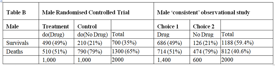
The result of the RCT on males when they were randomised to treatment is shown in Figure 3. This time were told that 70% of those with feature (s) who chose treatment in the Observational Study would have been the same in the RCT, so in the latter, P(y_t|s) = 0.7 and P(y’_t|s) = 0.3. From Bayes rule, P(s|y’_t) = 0.7x0.3/0.51 = 0.412 so that P(s‘|y’_t) = 0.588 and by Bayes rule again, P(s’|y’_t) = 0.51x0.588/0.3 = 1. This also means that P(s’∩y’_t) = 0.3*1 = 0.3 and from Figure 1, P(s’∩y’_c) = 0.09. In contrast to the female data, ‘benefit’ only occurs between {s∩y_t} and {s∩y_c} so for males if P(Benefit)=[P(s∩y_t)-P(s∩y_c)]=[0.49-0)=0.49, then p(Harm) = p(Benefit)-ATE=0.49-0.28=0.21

Figure 3: The results of randomisation to the treatment group in the RCT on males

Figure 3e

In the case of males, the reconstructed RCT result was very surprising. Many more men (actually 100%) were dying after treatment than on no treatment when it was 30% (exactly the same as in females). This suggested that the extra deaths on treatment were due to an adverse effect. It was also clear that none of those men surviving had taken the drug but all those dying had taken it. This would have been very noticeable to those conducting the RCT and would have prompted a detailed investigation leading to a discovery of the cause (e.g. anaphylaxis or fatal failure of an organ). Those males in the observational study would therefore have been forewarned not to take the drug unless they had the feature {s}.

The optimum strategy would therefore be to treat males with the feature {s} but not to treat those without that feature (i.e. s’). This means that a total of 49% would survive with {s} and being treated and a total of 21% with s’ and no treatment would survive giving a total of 49+21 = 70% surviving. If none of the men were treated 21% would survive. If they were all treated, 49% would survive. By contrast if all the females were treated, 49% would survive compared to 21% if none were treated. If only those females with {s} were treated 18.9% would survive together with 21% of those not treated giving as total of 39.9%. This is what happened in the observation study.

The CSM or FDA might license the treatment for all females but only the males with feature {s}.

1 Like