Should one derive risk difference from the odds ratio?

AndersHuitfeldt · April 2, 2023, 4:33pm

I have not yet decided how to respond to Suhail’s letter. I do however want to give some updates that may be of interest to readers of this thread:

Our preprint was discussed on Andrew Gelman’s blog at Count the living or the dead? | Statistical Modeling, Causal Inference, and Social Science , which led to some good discussion

A few days ago, Colnet et al posted a preprint on this issue to arXiv, at https://arxiv.org/pdf/2303.16008.pdf
This is a truly excellent paper, which provides several results that were not known to me, and presents the arguments with more precision and clarity than I have been able to. I think it is likely that many statistically inclined readers will find this to be much more convincing than our paper.

The Colnet et al preprint was also discussed on Gelman’s blog today, at “Risk ratio, odds ratio, risk difference… Which causal measure is easier to generalize?” | Statistical Modeling, Causal Inference, and Social Science

I encourage Suhail to re-evaluate whether he still stands by his letter, in light of Colnet et al.

s_doi · April 2, 2023, 8:14pm

They (Colnet et al) quote from my papers in addition to others but eventually conclude exactly what I said in 2013 in my JCE paper that I do not agree with anymore (scientific viewpoints are continually revised based on the accumulation of applied evidence on a scientific problem). Anyway the preprint has little bearing on the questions I raised in my letter and I look forwards to a robust response that is more applied than theoretical philosophy about what could be rather than what is.

f2harrell · April 2, 2023, 8:24pm

My current thinking is that one can (1) pick any model form they like and (2) use it too estimate any effect measure they like. That’s the spirit of this. It just happens that more than 1/2 of the time the logistic model is the most concise way to handle (1), i.e., the model that will need the fewest interaction terms. And I’ll be upfront in saying there is no universal theory to support this, just a lifetime of analyzing lots of datasets and looking a goodness of model fit.

Sander · April 2, 2023, 10:51pm

As you know, I have a very similar view. I would simply add some small technical amendments to your brief position summary, and make another semantic plea in the interest of encouraging better statistical interpretations among the mass of users (who do not read statistics blogs and whose grasp of statistical outputs hinges on words, not on math or even basic logic):

First, include proportional-hazards (Cox) and Poisson-regression models to reach well “over half the time”: Those models handle censored data more easily; true, they can be closely approximated by logistic models by entering time-varying intercepts in unconditional-logistic fitting or by conditioning on time strata in conditional-logistic fitting, but why bother with logistic models for censored data when software for PH fitting will automatically condition on exactly recorded times?

Second, the clear advantage of these statistically “natural” models over additive-risk or additive-rate models is their automatic obedience of logical range restrictions on risks and rates; I think that’s why you, me, and others have seen them require fewer product terms.

Third, I have long encouraged cessation of calling product terms “interactions”: Outside of very simplified cases (mostly involving additive models) they have no correspondence to concepts of mechanical interaction, and yet their presence or absence is often taken to signal presence or absence of mechanical interactions. Calling product terms “interactions” is even less defensible than calling P-values “significance levels” and calling inverted-P intervals “confidence intervals”. I realize of course these semantic mistakes of authorities are dismissed as minor or even defended by those wedded to them by tradition and their own past usage. But in my careful reading of the medical literature, their use has been and continues to be major sources of statistical misinterpretation - especially for those who cannot correctly grasp the mapping between the abstract statistical concepts and reality (which I think is the majority of researchers as well as readers).

f2harrell · April 2, 2023, 11:45pm

Well said Sander. Technical detail: I include more than simple products in many situations, i.e., allow nonlinear interactions. But more to your point I should label this as allowing for non-additivity on the current scale.

My comment about 1/2 of the time was referring to the binary Y situation.

Sander · April 3, 2023, 6:41pm

Thanks Frank. Regarding my item 3 to replace “interaction” with product term, some readers may find this review of interest:
Pearce, N., and Greenland, S. (2022). On the evolution of concepts of causal and preventive interdependence in epidemiology in the late 20th century | SpringerLink

On binary Y: As I’m sure you know, many analyses that focus on binary Y involve censored data (e.g., 5-year survival). Such data are selectively missing Y, with known missingness and outcome predictors in the form of the regression covariates and observation times. In that situation estimation of Y probabilities can be more efficient or less biased if done using a survival (failure-time) analysis rather than a logistic regression on the subset of data with Y known (which assumes censoring is uninformative and discards information from partial follow-up).

In this view, censored-survival methods are special types of methods for missing outcome data using various assumptions about the censoring process (from the stronger assumptions of conventional partial likelihood to the weaker assumptions of weighting proportional to inverse probability-of-censoring). That is why I emphasize including the logistic analogs for survival and person-time analyses when arguing for parsimony or stability, namely the Cox-PH and Poisson models for which the loglinear odds of the logistic model translates to loglinear hazards and loglinear rates (the models linear in the “natural” parameters and thus most well-behaved statistically), as they can outperform logistic modeling even if the target outcome is binary, and their software is just as well developed.

f2harrell · April 3, 2023, 7:30pm

Well put Sander. I was referring to the less common “true binary Y” case. To underscore one of your point, someone at my own institution a couple of months ago was ready to implement into EPIC a binary logistic regression model for disease development in 10 years where follow-up ranged from 0-10 years and censoring was not accounted for. They wanted to do this because they also entertained some machine learning methods that didn’t handle censoring that they ended up not using. I tried to explain the difficulty but it met deaf ears. I should have said this: I don’t know what you’re predicting with this model but it’s essentially the probability of disease development and having been admitted to hospital 5 years ago.

AndersHuitfeldt · April 21, 2023, 2:19pm

I am attaching here my draft response to Suhail Doi’s letter to the editor, which I plan to submit to the journal over the next few days. I would very much appreciate any feedback on this.

Dear Prof. Lash,

Prof. Doi is under the impression that the relative risk always varies with the baseline risk whereas the odds ratio does not. Further, he believes that these are universal mathematical properties of the effect measures, that hold true in any application.

It can easily be seen that no effect measure can be either universally baseline risk dependent or universally baseline risk independent. This depends on the data generating mechanism, which is usually not known a priori. However, if one effect measure is assumed to be homogeneous between groups, it will be possible to derive an explicit formula that relates the conditional value of another effect measure to the effect measure which is assumed to be stable. This formula will have a term for the baseline risk, which gives rise to appearance of baseline risk dependence relative to the model where another effect measure is stable. This phenomenon is symmetrical: The relative risk is baseline risk dependent relative to the model where the odds ratio is assumed to be homogeneous, and vice versa. The concept of relative baseline risk dependence is only of interest if it can be shown that an effect measure is baseline risk dependent or independent relative to the true data generating mechanism or relative to a generative model which accurately represents the relevant features of the data generating mechanism.

In order to formalize the intuition behind Sheps’ recommendations, I provided a plausible and biologically interpretable generative model that results in stability of her preferred variant of the relative risk (which depends on whether treatment increases or decreases risk). This relative risk is baseline risk independent relative to this generative model.

Because we do not have direct empirical access to the data generating mechanism, such work is by necessity theoretical. No claim is made that the generative model is always a correct representation of the data generating mechanism. Rather, its purpose is to provide an idealized scenario under which there would be homogeneity, such that any heterogeneity can be understood biologically in terms of deviation from the idealized model, with implications for how to reason about the required conditioning set (that is: which product terms must be included in a statistical model), and for sensitivity analysis.

Doi repeats his argument from elsewhere, which boils down to an observation that the odds ratio is baseline risk independent relative to a model where the ratio of likelihood ratios is stable between groups. This observation is not surprising, but only of interest if he can provide a biologically plausible generative model that results in stability of this ratio of likelihood ratios.

f2harrell · April 21, 2023, 2:54pm

This seems fair but ignores what tends to happen in the vast majority of real datasets.

s_doi · April 22, 2023, 8:39pm

This letter seems to me to be the same pattern of avoiding to respond directly to what has been written but go off on a tangent to argue about what I may be thinking. Not helpful at all in my humble opinion.

AndersHuitfeldt · April 22, 2023, 8:55pm

What specifically do you think I failed to respond to?

s_doi · April 28, 2023, 1:49pm

As I had posted earlier, we were working on indices of discrimination vis a vis odds ratios but then we realized something more illustrative that made that quest unimportant. I now post what we found.

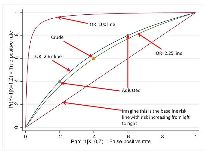
To begin, lets recap what we previously published (BMJ EBM) which is that if we take the binary outcome to be a test of the treatment status then we can interpret a clinical trial in diagnostic test terms. To explain this lets start with the figure below:

In the figure, the 45 degree line can be assumed to indicate baseline prevalence of the outcome increasing from left to right. We can then draw curves where the ratio of true positive probability (TPR) to false positive probability (FPR) is a constant on the odds scale and three such “constancy curves” are depicted in the figure (ratios of 2.25, 2.67 and 100). On these curves, the actual TPRs and FPRs vary but their ratios as odds do not.

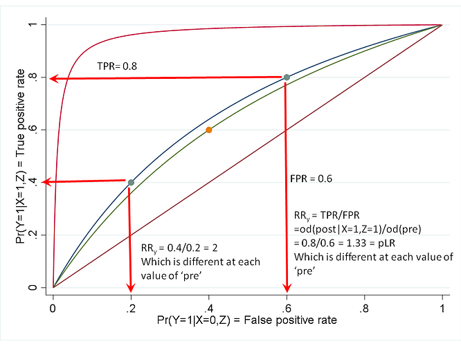
Now lets take a look at a second figure below:

The 2.25 curve is from a crude analysis of exposure and outcome with the actual FPR and TPR indicated (by the marker) from the study. The 2.67 curve is from a stratified analysis by a prognostic non-confounding variable Z and the markers indicate the FPR and TPR when Z=0 or Z=1.

What is interesting is that from Bayes’ theorem, TPR/FPR is nothing more than the od(post|X=1)/od(pre) and therefore their ratio is conditional on baseline prevalence ‘pre’ and the latter is known as the relative risk (RR). Since this is conditional on ‘pre’ the RR is mathematically dependent on baseline prevalence.

The ratio of od(TPR)/od(FPR) = odds ratio (OR) and as is evident in the figures with ‘constancy curves’ has no relationship to baseline prevalence. This is because:
OR = [od(post|X=1)/od(pre)] / [od(post|X=0)/od(pre)]
and therefore ‘od(pre)’ cancels out
This is an elegant confirmation that requires neither simulation nor abstract theorization and look forward to thoughts from @Sander as if this holds then there is no need for us to debate the issue of mathematical portability of these effect measures henceforth since the RR is clearly non-portable and the OR is portable across baseline prevalence of an outcome (such prevalence usually aligning with severity of disease).

NB updated to remove typos and graphical errors
NB2 updated “portability” to “mathematical portability” for clarity and to distinguish this from generalizability

Sander · April 28, 2023, 5:52pm

“…and the OR is portable across baseline prevalence of an outcome…” As far as I can see, that statement is a non-sequitur and foregone conclusion that recurs throughout your posts and papers on this topic, along with other logical fallacies and easily refutable assertions. I’ll try to summarize the major ones:

The matter of portability is in the end empirical. Anyone can look at real study reports to see how measures vary across studies. Provided that one does not commit the nullistic fallacy of confusing p>0.05 with absence of variation, it is easy to see that all measures usually vary quite a bit across baseline risks, which is often just as expected from knowledge of the underlying causal mechanisms. That the OR might vary less could just as well be taken as a defect of the OR for some purposes, insofar as baseline risks are of crucial practical importance in many if not most real applications.

To assert empirical claims like “…and the OR is portable across baseline prevalence of an outcome…” based on math results is an example of reification of abstractions that at best are theories or hypotheses that need to be evaluated against data. Empirical studies have been done by different parties and some have noted how others commit further fallacies by declaring greater portability for ORs based on statistics that are incommensurable across measures.

The ultimate fallacy in the quoted claim is however the degradation of a defensible (albeit still empirical) thesis, “by some criteria, the OR tends to be more portable than the RR”, into the flat assertion that “…the OR is portable across baseline prevalence of an outcome…”, which is simply false: Put random positive numbers that sum to 1 into a series of 2x2 tables to create a hypothetical set of expected counts, and you will almost surely see variation across the tables in both baseline prevalence and every measure, including the OR.

As usual, my practical views aren’t very far from Frank’s, experience being a potent source of convergence, and I have already explained them at length in this thread and others over the years here on Datamethods. First, variation dependence among parameters can contribute to heterogeneity via range restrictions. Risk ratios have that heterogeneity source when the outcome becomes common enough in some comparison groupings; the source is even stronger for risk differences. In contrast, odds ratios and hazard rate ratios do not have that mathematical source of heterogeneity. But there are many real-world sources of heterogeneity that affect all measures; most of them are uncontrolled in real study reports and usually unmeasured in real data sets. Thus there is no compelling case for ignoring heterogeneity in any measure, other than simple inability to estimate it reliably with available data.

The ubiquity of heterogeneity as well as cost-benefit considerations show that we need to focus on estimating practice-relevant features of entire conditional distributions of multivariate outcomes, at least if we are concerned with addressing medical problems rather than math problems. Every summary measure is deficient and potentially misleading for practical purposes because it ignores or discards important information. You shouldn’t buy a car based on its horsepower alone, nor should you buy a cancer treatment based on a summary measure of 5-year survival alone - after all what if it extends your life 4 years, but those 4 years are as locked-in paralysis?

For all these reasons and others I have discussed here over what is now years, I find your obsession with promoting ORs misguided at best, and misleading if taken seriously. Where we may agree is this: Suppose one knows nothing about the causal mechanisms to suggest a particular model and (as always) the data are too limited to approach the above-stated ideal. Then, for statistical stability and simplicity reasons, it makes sense to use a model form linear in the natural parameter of the data distribution (logistic for risks, loglinear for counts and hazard rates, etc.) that obeys the logical range restrictions of the outcome. This choice makes the usual large-sample approximations (e.g., Wald P-values and CIs) most accurate in finite samples, and in the logistic case makes ORs the easiest summary measures to calculate. What it emphatically does not do is make the OR the most relevant measure in any contextual, scientific, policy or medical sense. For those real-world purposes the ideal target is again the entire conditional multivariate distribution of the outcomes of concern, and any summary measure can lead to distorted inferences and bad decisions due to overlooking the information the summary disregards.

s_doi · April 28, 2023, 9:46pm

Thanks for your prompt response and I would, of course, agree with you had we been discussing transportability (i.e. generalizability) of causal effects - however this is not what I am talking about in my post.

Mathematical portability (the influence of baseline prevalence on the ability of a computed effect to measure the magnitude of association correctly) does not need any consideration of random nor systematic error. It is just referring to whether the effect measure’s computed value can be shown to change for reasons other than the XY association (in this case the reason being investigated is baseline prevalence).

This concept does not need to be evaluated against real world data since I am not arguing for greater generalizability for OR’s in my post. The distinction you make between “by some criteria, the OR tends to be more portable than the RR”, and “…the OR is portable across baseline prevalence of an outcome…” suggests that you are referring to generalizability here and given the numerical similarity between OR and RR especially at smaller baseline prevalence I am quite sure that you are quite right about their equivalent transportability in the real world. I therefore fully agree with you that if we were to “put random positive numbers that sum to 1 into a series of 2x2 tables to create a hypothetical set of expected counts” we would certainly see “variation across the tables in both baseline prevalence and every measure, including the OR” but this is a different issue from its mathematical ability to measure what it is intended to measure.

There are many other areas (other than generalizability) where these mathematical properties would become important, but perhaps that can be left for a later discussion. Right now, I am seeking agreement on the mathematics outlined above and if there is no flaw to be pointed out, and there is broad agreement, then we can move on to these other issues.

Sander · April 29, 2023, 5:14am

As far as I can tell, all you’ve done with your math is reframe the long-known mathematical facts that the OR is variation independent of the designated baseline (reference) risk, while the RR isn’t (nor is the RD). You seem to call the OR result “portability”; I object to that usage because in ordinary English portability is a synonym for transportability, and there is already an unambiguous and established math term for what you describe: variation independence (VI), which is also called mathematical or logical independence (as opposed to statistical independence, which can occur with or without VI).

In another misuse of terms, you seem to confuse outcome incidence probability (risk) with outcome prevalence; with rare exceptions, trials examine risk, not prevalence.

I explained in my last post what VI does and doesn’t mean for practice. In particular, the fact that the OR is variation independent of baseline risk can be seen as a disadvantage in some contexts. Even when this VI is seen as an advantage because it eliminates a source of effect-measure heterogeneity, it does not address causally important sources such as variation in patient response.

I repeat from a much earlier post that the RR is variation independent of a parameter different from baseline risk, the log of the odds product or equivalently, the sum of the logits. This fact leads to a modeling and estimation approach which has some advantages over maximum-likelihood logistic regression; see Richardson, Robins & Wang, ‘On Modeling and Estimation for the Relative Risk and Risk Difference’, JASA 2017.

I will try to avoid posting back further on this issue as I have written out all the facts as I understand them, and have unrelated items to attend to. I hope others will take over responding to you, whether or not they share your or my view.

s_doi · April 29, 2023, 11:33am

Thanks for your further thoughts on this matter. Regarding the specific points you raise, I used portability instead of variation independence (VI) because I thought it would be easier for clinicians to comprehend and a series of my papers have used this (even in the titles, not just the text) so probably need to be consistent. However point taken and for epidemiology readers will add ‘mathematical portability is also known as VI and does not imply generalizability or transportability as used in epidemiology’ in parentheses.
Regarding incidence or risk instead of prevalence – I use the term prevalence to refer to a dataset, and this can be from a trial or from other designs. At the end of follow-up we have a certain prevalence of the outcome in the entire dataset. The reason I have tried to avoid risk is that this is then confused with baseline risk (in the control group for example) but the variation or mathematical independence is actually linked to prevalence of the outcome in the dataset being analysed (or its subset) not to baseline risk. Of course baseline risk is associated with such prevalence so sometimes we loosely say independence from baseline risk but when the actual math is being discussed, I think its more accurate to use ‘prevalence in a dataset’ but point taken, will add ‘prevalence in a dataset’ to future discussions. I agree fully that VI adds unnecessary heterogeneity and confusion to the effect measure but of course has nothing to do with real world sources of confusion and heterogeneity such as variations in levels of care or heterogeneity in patient response.
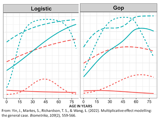
I note that you have mentioned the generalized log odds product model previously and the log(odds product) is just logit(TPR)+logit(FPR) in my diagram above. It was made popular in the earlier days for summarizing ROC curves (now superseded by HSROC or SCS models). I really do not see why that should work better than predicted probabilities from logistic models – except when one is determined to only model the RR and nothing else. The authors of the generalized odds product model have reported a comparison of predicted probabilities using the Titanic data. Their dataset consisted of 1309 passengers from three passenger classes, of whom 809 lost their lives during the event. They removed the 263 (20:1%) passengers for whom age was missing, resulting in a sample size of 1046, including 284 (27:1%) passengers in the first class, 261 (25:0%) in the second class, and 501 (47:9%) in the third class. Predicted probability of death of the first passenger class (solid line), the second class (dotted line), and the third class (dashed line) with respect to different models are indicated in the figure below (red represents female, and blue represents male).

I do not find the differences in predicted probability by the GOP model as more sensible from first principles regarding the logical representation of the events that unfolded suggesting that there could be bias in inference through this model – this dataset is freely available and others can do the analysis (brm-package in R) and see for themselves what they think.

No worries, it will be interesting to see what others think as well so will leave this without asking further questions for 1-2 weeks.

Addendum: I could not replicate the Yin et al results and my analysis is below. Circles are class 1 F, diamonds are class 2 F, triangles are class 1 M, squares class 3 F. The other two on top are class 2 & 3 M.

AndersHuitfeldt · April 29, 2023, 3:18pm

I would like to make the following points:

(1) The switch relative risk is variation independent of the baseline risk, in the sense defined by Richardson, Wang and Robins (2017): The range of possible values of (SRR(v), P0(v)) is equal to the Cartesian product of the ranges of SRR(v) and P0(v).

(2) “Variation independence” is very closely related to what I have called “closure” of an effect measure. To recap, closure means that for any (conditional) baseline risk in [0,1] and for any possible value of the (conditional) effect measure, the implied (conditional) risk under treatment is also in [0,1]. It seems likely to me that closure is equivalent to variation independence, or at least that the definitions coincide for all standard effect measures.

(3) I will apologise in advance for making a point about semantics: While the term “variation independent” points to a mathematically reasonable referent, the term itself is in my view misnomer, and will give rise to misunderstandings, as is readily apparent in Suhail’s response.

To recap the recent history of this discussion: I wrote a commentary on the contributions of Mindel Sheps, in which I noted “closure” as a relevant consideration. Suhail responded with a letter to the editor where he argued that closure is not the main consideration, but that what actually matters is “baseline risk independence”. If we now agree that the concept Suhail is pointing towards is “variation independence”, that variation independence is essentially the same thing as closure, and that closure is a property of the switch relative risk: Can we then agree, to borrow a phrasing from earlier in this thread, that this brings closure to the issue?

Sander · April 29, 2023, 4:19pm

Thanks Anders, I had you most in mind in asking others to comment…

Re your 2: Yes your “closure” is equivalent to VI for risk and measures of association of treatment with risk. VI is not a causal concept and it applies whether those measures are of effects or not; the math goes through without specifying an underlying causal model.

Re 3: You did not explain how “variation independent” is a misnomer. As far as I can see the term is unambiguous and I do not see how the term could be mistaken for something else. So how is VI a misnomer? I could see the term as sounding too technical, and another equivalent term like “range independence” might be clearer to most readers. Still, VI is precise and has an established usage over generations of math stat.

In contrast, “closure” already has established uses for other, unrelated concepts such as the combination of a region and its boundary, and a specific statement formed by binding all free variables in an expression. Thus, as with “consistency”, “closure” risks confusion should the different concepts with the same label arise in the same discussion. Also notable is how your comment ends by invoking yet another meaning of “closure”. So if you use “closure” in teaching I would advise cautioning that it has multiple technical as well as ordinary English meanings.

R_cubed · April 30, 2023, 12:02pm

It seems like there is a general agreement that no modelling strategy dominates others in all cases. So while there may be reasonably strong prior (or expert) information that suggests the logistic model is a good default (ie. the opinion of @f2harrell ), it might not reflect all uncertainty that a skeptical audience might have (@AndersHuitfeldt).

Wouldn’t a principled way to decide this issue be based on model averaging or model selection techniques whether Bayesian or Frequentist? How would someone specify the data analysis plan for this methodology?

I ask this after looking at the application of Bayesian Model Averaging to the issue of fixed vs random effect meta-analysis, and came across this R package: metaBMA: Bayesian (or Frequentist) Model Averaging for Fixed and Random Effects Meta-Analysis.

Related Threads: